You are viewing the documentation for an older COMSOL version. The latest version is available here.
PDF

Shock Response of a Motherboard
Introduction
Electronic equipment often has to certified to function after having been subjected to a specified shock loading. Performing a numerical simulation is cheaper, and has a lower turnaround time, than doing the actual physical testing. In many cases, it is not necessary to perform a full nonlinear contact analysis. Rather, the requirement is specified in terms of a certain given acceleration history.
A common such specification of a shock is that the acceleration behaves as a half sine function with a given period and peak amplitude.
In this example, the effect of a 50g half-sine shock load with a duration of 11 ms on a computer motherboard is investigated using two approaches: response spectrum analysis and direct time stepping using mode superposition.
Model Definition
GEOMETRY
Figure 1 shows a motherboard with a design that is typical for smaller computer devices such as game consoles, for example.
Figure 1: Motherboard geometry.
A processor (CPU) and a graphics chip (GPU) are covered by massive heat sinks used for passive cooling. Memory chips are located next to the CPU unit. A number of cylindrical capacitors of various sizes are scattered over the motherboard. Several connectors for peripherals are located along the motherboard edges. The board is attached to the housing via six mounting bolts. The latter are not modeled explicitly.
Material
The board itself is made of a generic PCB material. The heat sinks are made of aluminum. The chips are modeled as made of silicon. The connectors are modeled as rectangular blocks made of plastic. Some effective material properties are used to represent the capacitors.
Constraints
All six mounting holes have fixed constraints on their cylindrical boundaries.
Loads
For the response spectrum analysis, the loading is represented by a pseudoacceleration spectrum as shown in Figure 2.
Figure 2: Vertical spectrum for 50g shock load with 11 ms duration.
During the transient computations, all parts of the motherboard are subjected to a transient body load (gravity load) with 50g magnitude and 11 ms duration:
(1)
Mesh
Figure 3 shows the mesh used.
Figure 3: Mesh.
The discretization using this mesh together with quadratic serendipity elements results in approximately 100,000 degrees of freedom (DOF) being used in the eigenfrequency analysis.
Results and Discussion
As a first step, the lowest fifteen eigenfrequencies have been computed. Figure 4 shows their distribution together with the values of the participation factors for the corresponding eigenmodes.
Figure 4: Participation factors for Z-translation for all the eigenmodes.
The sum of the effective modal mases for all computed eigenmodes is around 0.94. Thus, the modes account for about 94% of the vertical dynamic forces of the system.
Figure 5 shows the values of the vertical shock spectrum computed at the eigenfrequencies.
Figure 5: Vertical shock spectrum input at eigenfrequencies.
Thus, the first and third modes have the largest participation factor for vertical translation. The eigenfrequency for the third mode is also located close to the maximum of the input spectrum, so these two modes seem important for the response. The modes are shown in Figure 6 and Figure 7 below.
Figure 6: The 1st eigenmode.
Figure 7: The 3rd eigenmode.
The response spectrum evaluation is based on the eigenvalue solution, and it is performed during postprocessing using a dedicated dataset called Response Spectrum.
In Figure 8, the vertical displacement response, as computed using the CQC mode combination method with damping of 5% is shown.
Figure 8: Vertical displacement, as a result of the response spectrum evaluation.
Figure 9 shows the stress distribution computed using the response spectrum analysis. The plot shows rather high stress level at the memory chips.
Figure 9: Stress in the motherboard components.
For comparison, the same analysis is also performed in the time domain, using a Time Dependent, Modal solver. Figure 10 shows the vertical displacement of the system after 11 ms of transient loading.
Figure 10: Dynamic response of the system at the end of the shock pulse.
The maximum displacement computed over a 60 ms long transient simulation is shown in Figure 11.
Figure 11: Maximum vertical displacement.
Note that the maximum is computed pointwise, so that Figure 11 does not correspond to a state of the system at some particular time instance. Rather, it gives an estimation of the worst deformation response in each point. In this sense, the plot presents a similar information as the computations of the shock spectrum response, and can be compared with Figure 8. Both methods indicate a maximum displacement of about 8 mm.
Notes About the COMSOL Implementation
The two methods used here has different merits. The response spectrum method only provides an approximate solution, whereas the time stepping is exact (within the limits given by time discretization and truncation of higher modes). On the other hand, you will have to store a full solution for all time steps in order to find the maximum values when using time stepping. This will cause large file sizes.
Note that the maximum response can occur significantly later than the end of the shock, particularly for systems with low damping. During the time stepping, a few periods of the lowest eigenfrequency should be covered. Here, the end of the time stepping is set to 60 ms, which is about three full periods of the first eigenmode.
For the time-dependent analysis, you enter the function for the load by entering the factor:
50*sin(2*pi/22[ms]*t)*(t<11[ms]) in the Load factor input field available in the Modal Solver node’s settings. The body load set up via the Gravity node will be multiplied by this factor, giving an effective load magnitude of 50g.
Application Library path: Structural_Mechanics_Module/Dynamics_and_Vibration/motherboard_shock_response
Modeling Instructions
From the File menu, choose New.
New
In the New window, click  Model Wizard.
Model Wizard
1
In the Model Wizard window, click  3D.
2
In the Select Physics tree, select Structural Mechanics>Solid Mechanics (solid).
3
Click Add.
4
Click  Study.
5
In the Select Study tree, select Preset Studies for Selected Physics Interfaces>Response Spectrum.
6
Geometry 1
Import the motherboard geometry from a file.
Import 1 (imp1)
1
In the Home toolbar, click  Import.
2
In the Settings window for Import, locate the Import section.
3
Click  Browse.
4
5
Click  Import.
Form Union (fin)
1
In the Model Builder window, under Component 1 (comp1)>Geometry 1 click Form Union (fin).
2
In the Settings window for Form Union/Assembly, locate the Form Union/Assembly section.
3
From the Action list, choose Form an assembly.
4
In the Home toolbar, click  Build All.
5
Click the  Go to Default View button in the Graphics toolbar.
The imported geometry should look similar to that shown in Figure 1.
Definitions
Prepare selections of the motherboard components to simplify the modeling process.
PCB
1
In the Definitions toolbar, click  Explicit.
Select the printed circuit board.
2
3
In the Settings window for Explicit, type PCB in the Label text field.
Heat sinks
1
In the Definitions toolbar, click  Explicit.
Select both heat sinks.
2
3
In the Settings window for Explicit, type Heat sinks in the Label text field.
Chips
1
In the Definitions toolbar, click  Explicit.
Select the CPU, GPU, and memory chips.
2
3
In the Settings window for Explicit, type Chips in the Label text field.
Connector blocks
1
In the Definitions toolbar, click  Explicit.
Select all seven connector blocks located along the edges of the board.
2
3
In the Settings window for Explicit, type Connector blocks in the Label text field.
Capacitors (larger)
1
In the Definitions toolbar, click  Explicit.
Select five capacitors of larger size placed in a row next to one of the heat sinks.
2
3
In the Settings window for Explicit, type Capacitors (larger) in the Label text field.
Capacitors (smaller)
1
In the Definitions toolbar, click  Explicit.
Select all the remaining capacitors that are scattered over the motherboard.
2
3
In the Settings window for Explicit, type Capacitors (smaller) in the Label text field.
Mounting holes
1
In the Definitions toolbar, click  Explicit.
Select the boundaries for all six mounting holes. You can use the Select Box button to select one hole at a time and add its selection, then proceed to the next one.
2
In the Settings window for Explicit, locate the Input Entities section.
3
From the Geometric entity level list, choose Boundary.
4
5
In the Label text field, type Mounting holes.
View 1
1
In the Model Builder window, under Component 1 (comp1)>Definitions click View 1.
2
In the Settings window for View, locate the Colors section.
3
Select the Show material color and texture check box.
Add Material
1
In the Home toolbar, click  Add Material to open the Add Material window.
2
Go to the Add Material window.
3
In the tree, select Built-in>FR4 (Circuit Board).
4
Right-click and choose Add to Component 1 (comp1).
Materials
FR4 (Circuit Board) (mat1)
1
In the Model Builder window, under Component 1 (comp1)>Materials click FR4 (Circuit Board) (mat1).
2
In the Settings window for Material, locate the Geometric Entity Selection section.
3
From the Selection list, choose PCB.
Add Material
1
Go to the Add Material window.
2
In the tree, select Built-in>Aluminum.
3
Right-click and choose Add to Component 1 (comp1).
Materials
Aluminum (mat2)
1
In the Model Builder window, under Component 1 (comp1)>Materials click Aluminum (mat2).
2
In the Settings window for Material, locate the Geometric Entity Selection section.
3
From the Selection list, choose Heat sinks.
Add Material
1
Go to the Add Material window.
2
In the tree, select Built-in>Silicon.
3
Right-click and choose Add to Component 1 (comp1).
Materials
Silicon (mat3)
1
In the Model Builder window, under Component 1 (comp1)>Materials click Silicon (mat3).
2
In the Settings window for Material, locate the Geometric Entity Selection section.
3
From the Selection list, choose Chips.
Add Material
1
Go to the Add Material window.
2
In the tree, select Built-in>Acrylic plastic.
3
Right-click and choose Add to Component 1 (comp1).
Materials
Acrylic plastic (mat4)
1
In the Model Builder window, under Component 1 (comp1)>Materials click Acrylic plastic (mat4).
2
In the Settings window for Material, locate the Geometric Entity Selection section.
3
From the Selection list, choose Connector blocks.
4
Click to expand the Appearance section. From the Material type list, choose Plastic (shiny).
5
From the Color list, choose Black.
Cylindrical capacitors have a complex internal structure with several layers of different materials. For the effective material, use the same elasticity moduli as for aluminum, which is the material of the capacitor’s outer cylinder.
Add Material
1
Go to the Add Material window.
2
In the tree, select Built-in>Aluminum.
3
Right-click and choose Add to Component 1 (comp1).
Materials
Capacitors (larger) composite material
1
In the Model Builder window, under Component 1 (comp1)>Materials click Aluminum 1 (mat5).
2
In the Settings window for Material, type Capacitors (larger) composite material in the Label text field.
3
Locate the Geometric Entity Selection section. From the Selection list, choose Capacitors (larger).
Set the effective material density for the larger capacitors.
4
Locate the Material Contents section. In the table, enter the following settings:
Keep all the other mechanical properties the same as for aluminum.
5
Click to expand the Appearance section. From the Material type list, choose Plastic (shiny).
6
From the Color list, choose Yellow.
Add Material
1
Go to the Add Material window.
2
In the tree, select Built-in>Aluminum.
3
Right-click and choose Add to Component 1 (comp1).
4
In the Home toolbar, click  Add Material to close the Add Material window.
Materials
Capacitors (smaller) composite material
1
In the Settings window for Material, locate the Geometric Entity Selection section.
2
From the Selection list, choose Capacitors (smaller).
3
In the Label text field, type Capacitors (smaller) composite material.
Set the effective material density for the larger capacitors.
4
Locate the Material Contents section. In the table, enter the following settings:
5
Click to expand the Appearance section. From the Material type list, choose Plastic (shiny).
6
From the Color list, choose Cyan.
Solid Mechanics (solid)
Fixed Constraint 1
1
In the Model Builder window, under Component 1 (comp1) right-click Solid Mechanics (solid) and choose Fixed Constraint.
2
In the Settings window for Fixed Constraint, locate the Boundary Selection section.
3
From the Selection list, choose Mounting holes.
Mesh 1
Size 1
1
In the Model Builder window, under Component 1 (comp1) right-click Mesh 1 and choose Size.
Explicitly prescribe the mesh size for the domains representing smaller capacitors.
2
In the Settings window for Size, locate the Geometric Entity Selection section.
3
From the Geometric entity level list, choose Domain.
4
From the Selection list, choose Capacitors (smaller).
5
Locate the Element Size section. From the Predefined list, choose Fine.
Free Quad 1
1
In the Mesh toolbar, click  Boundary and choose Free Quad.
Select one side boundary of each heat sink together with the top boundary of the PCB for quad meshing. This is to control the directions of the mesh sweep that you set up in the coming modeling steps.
2
Size 1
1
Right-click Free Quad 1 and choose Size.
2
In the Settings window for Size, locate the Geometric Entity Selection section.
3
From the Selection list, choose All boundaries.
4
Locate the Element Size section. From the Predefined list, choose Extremely fine.
5
Click the Custom button.
6
Locate the Element Size Parameters section. Select the Maximum element size check box.
7
8
Select the Minimum element size check box.
Mapped 1
1
In the Mesh toolbar, click  Boundary and choose Mapped.
Do a similar thing using mapped meshes on the top boundaries of all rectangular components. You might need to hide the heat sink domains to select the top boundaries of the CPU and GPU components.
2
Size 1
1
Right-click Mapped 1 and choose Size.
2
In the Settings window for Size, locate the Geometric Entity Selection section.
3
From the Selection list, choose All boundaries.
4
Locate the Element Size section. From the Predefined list, choose Extra fine.
Swept 1
In the Mesh toolbar, click  Swept.
Distribution: Default
1
Right-click Swept 1 and choose Distribution.
2
In the Settings window for Distribution, type Distribution: Default in the Label text field.
3
Locate the Distribution section. In the Number of elements text field, type 3.
Distribution: PCB
1
In the Model Builder window, right-click Swept 1 and choose Distribution.
2
In the Settings window for Distribution, type Distribution: PCB in the Label text field.
3
Locate the Domain Selection section. From the Selection list, choose PCB.
4
Locate the Distribution section. In the Number of elements text field, type 2.
Distribution: Heat sinks
1
Right-click Swept 1 and choose Distribution.
2
In the Settings window for Distribution, type Distribution: Heat sinks in the Label text field.
3
Locate the Domain Selection section. From the Selection list, choose Heat sinks.
4
Locate the Distribution section. In the Number of elements text field, type 4.
5
Click  Build All.
6
Click the  Go to Default View button in the Graphics toolbar.
The final mesh should look similar to that shown in Figure 3.
Global Definitions
Acceleration (g) vs. Frequency (Hz)
1
In the Home toolbar, click  Functions and choose Global>Interpolation.
2
In the Settings window for Interpolation, type Acceleration (g) vs. Frequency (Hz) in the Label text field.
3
Locate the Definition section. Click  Load from File.
4
Vertical Spectrum
1
In the Home toolbar, click  Functions and choose Global>Analytic.
2
In the Settings window for Analytic, type Vertical Spectrum in the Label text field.
3
In the Function name text field, type vsp.
4
Locate the Definition section. In the Arguments text field, type freq.
5
In the Expression text field, type int1(freq)*g_const.
6
Locate the Units section. In the table, enter the following settings:
7
In the Function text field, type m/s^2.
8
Locate the Plot Parameters section. In the table, enter the following settings:
9
Click  Create Plot.
Results
Vertical Spectrum
1
In the Settings window for 1D Plot Group, type Vertical Spectrum in the Label text field.
2
Locate the Plot Settings section. Select the x-axis label check box.
3
4
Select the y-axis label check box.
5
In the associated text field, type Pseudoacceleration (m/s^2).
6
Locate the Axis section. Select the Manual axis limits check box.
7
In the x minimum text field, type 0.
8
In the x maximum text field, type 600.
9
In the Vertical Spectrum toolbar, click  Plot.
Study 1
Step 1: Eigenfrequency
1
In the Model Builder window, under Study 1 click Step 1: Eigenfrequency.
2
In the Settings window for Eigenfrequency, locate the Study Settings section.
3
From the Eigenfrequency search method list, choose Manual.
4
Select the Desired number of eigenfrequencies check box.
5
6
Select the Search for eigenfrequencies around check box.
7
8
In the Home toolbar, click  Compute.
Results
Mode Shape (solid)
1
Click the  Go to Default View button in the Graphics toolbar.
The default plot shows the eigenmode shape for the first natural frequency.
Evaluate the participation factors for vertical translation for all computed eigenmodes.
Table
1
Go to the Table window.
2
Click Table Graph in the window toolbar.
Results
Table Graph 1
1
In the Model Builder window, under Results>1D Plot Group 3 click Table Graph 1.
2
In the Settings window for Table Graph, locate the Data section.
3
From the Plot columns list, choose Manual.
4
In the Columns list, select Participation factor, normalized, Z-translation (1).
5
Locate the Coloring and Style section. Find the Line markers subsection. From the Marker list, choose Asterisk.
6
From the Positioning list, choose In data points.
7
Find the Line style subsection. From the Line list, choose Dotted.
Participation Factors
1
In the Model Builder window, under Results click 1D Plot Group 3.
2
In the Settings window for 1D Plot Group, type Participation Factors in the Label text field.
Also evaluate the values of the shock spectrum input at all computed eigenfrequencies.
Vertical Spectrum
1
In the Model Builder window, click Vertical Spectrum.
2
In the Settings window for 1D Plot Group, locate the Axis section.
3
In the x minimum text field, type 30.
4
In the x maximum text field, type 400.
5
In the y minimum text field, type 500.
6
In the y maximum text field, type 850.
7
Locate the Legend section. From the Position list, choose Middle right.
Global 1
1
Right-click Vertical Spectrum and choose Global.
2
In the Settings window for Global, locate the Data section.
3
From the Dataset list, choose Study 1/Solution 1 (sol1).
4
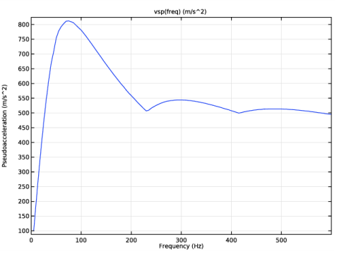
Click Replace Expression in the upper-right corner of the y-Axis Data section. From the menu, choose Global definitions>Functions>vsp(freq) - Vertical Spectrum.
5
Locate the x-Axis Data section. From the Parameter list, choose Expression.
6
In the Expression text field, type freq.
7
Click to expand the Coloring and Style section. Find the Line style subsection. From the Line list, choose None.
8
Find the Line markers subsection. From the Marker list, choose Cycle.
9
From the Positioning list, choose In data points.
10
Click to expand the Legends section. From the Legends list, choose Manual.
11
12
In the Vertical Spectrum toolbar, click  Plot.
Note that the third eigenmode has the maximum participation factor for vertical translation. It is also close to the maximum of the shock spectrum input. Plot this eigenmode.
Mode Shape (solid)
1
In the Model Builder window, under Results click Mode Shape (solid).
2
In the Settings window for 3D Plot Group, locate the Data section.
3
From the Eigenfrequency (Hz) list, choose 68.551.
4
In the Mode Shape (solid) toolbar, click  Plot.
5
Click the  Go to Default View button in the Graphics toolbar.
As a final check, calculate the sum of relative modal masses for all computed eigenmodes.
Global Evaluation 1
1
In the Results toolbar, click  Global Evaluation.
2
In the Settings window for Global Evaluation, click Replace Expression in the upper-right corner of the Expressions section. From the menu, choose Component 1 (comp1)>Definitions>Response Spectrum 1>Effective modal mass>rsp1.mEffLZ - Effective modal mass, Z-translation - kg.
3
Locate the Expressions section. In the table, enter the following settings:
4
Locate the Data Series Operation section. From the Transformation list, choose Integral.
5
From the Method list, choose Summation.
6
Clicknext to  Evaluate, then choose New Table.
The value shows that the computed eigenmodes account for more than 94% of the total mass.
Add a special dataset for response spectrum evaluation.
Response Spectrum 3D 1
1
In the Results toolbar, click  More Datasets and choose Response Spectrum 3D.
2
In the Settings window for Response Spectrum 3D, locate the Spectra section.
3
From the Vertical spectrum list, choose Vertical Spectrum (vsp).
Maximum Displacement, Response Spectrum
1
In the Results toolbar, click  3D Plot Group.
2
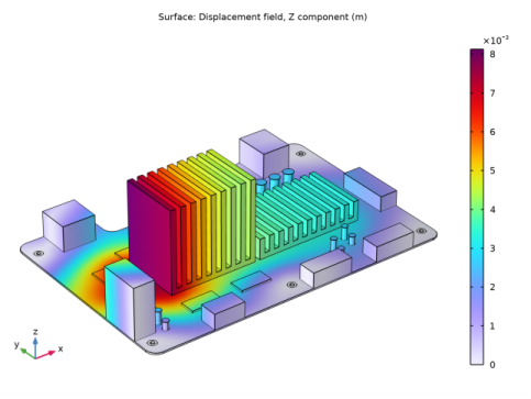
In the Settings window for 3D Plot Group, type Maximum Displacement, Response Spectrum in the Label text field.
3
Locate the Data section. From the Dataset list, choose Response Spectrum 3D 1.
Surface 1
1
Right-click Maximum Displacement, Response Spectrum and choose Surface.
2
In the Settings window for Surface, locate the Expression section.
3
In the Expression text field, type w.
4
Locate the Coloring and Style section. From the Color table list, choose Prism.
5
In the Maximum Displacement, Response Spectrum toolbar, click  Plot.
6
Click the  Go to Default View button in the Graphics toolbar.
Solid Mechanics (solid)
Next, perform a transient analysis of the structure response under a body load in the form of a half-sine pulse with 11 ms duration and 50 g magnitude.
Gravity 1
1
In the Physics toolbar, click  Domains and choose Gravity.
2
In the Settings window for Gravity, locate the Domain Selection section.
3
From the Selection list, choose All domains.
Use a Time Dependent, Modal solver, which computes the transient response by representing the solution as a superposition of precomputed eigenmodes.
Add Study
1
In the Home toolbar, click  Add Study to open the Add Study window.
2
Go to the Add Study window.
3
Find the Studies subsection. In the Select Study tree, select Empty Study.
4
5
In the Home toolbar, click  Add Study to close the Add Study window.
Study 2
1
In the Settings window for Study, locate the Study Settings section.
2
Clear the Generate default plots check box.
Time Dependent, Modal
1
In the Study toolbar, click  Study Steps and choose Time Dependent>Time Dependent, Modal.
2
In the Settings window for Time Dependent, Modal, locate the Study Settings section.
3
From the Time unit list, choose ms.
4
In the Output times text field, type range(0,0.5,60).
5
From the Tolerance list, choose User controlled.
6
In the Relative tolerance text field, type 0.0001.
Solution 2 (sol2)
1
In the Study toolbar, click  Show Default Solver.
2
In the Model Builder window, expand the Solution 2 (sol2) node, then click Modal Solver 1.
3
In the Settings window for Modal Solver, locate the Eigenpairs section.
4
From the Solution list, choose Solution 1 (sol1).
5
In the Damping ratios text field, type 0.05.
6
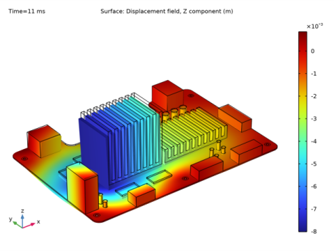
Click to expand the Advanced section. In the Load factor text field, type 50*sin(2*pi/22[ms]*t)*(t<11[ms]).
This factor multiplies all applied loads, including the gravity load.
7
Click to expand the Output section. Not storing the time derivative reduces the size of the output data.
8
Clear the Store time derivatives check box.
9
In the Study toolbar, click  Compute.
Results
Maximum Displacement, Time History
1
In the Home toolbar, click  Add Plot Group and choose 3D Plot Group.
2
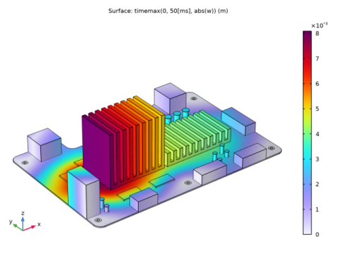
In the Settings window for 3D Plot Group, type Maximum Displacement, Time History in the Label text field.
3
Locate the Data section. From the Dataset list, choose Study 2/Solution 2 (sol2).
Surface 1
1
Right-click Maximum Displacement, Time History and choose Surface.
2
In the Settings window for Surface, locate the Expression section.
3
In the Expression text field, type timemax(0,60[ms],abs(w)).
4
Locate the Coloring and Style section. From the Color table list, choose Prism.
Maximum Displacement, Time History
1
In the Model Builder window, click Maximum Displacement, Time History.
2
In the Settings window for 3D Plot Group, click to expand the Title section.
3
From the Title type list, choose Manual.
4
In the Title text area, type Surface: timemax(0, 50[ms], abs(w)) (m).
5
Clear the Parameter indicator text field.
6
In the Maximum Displacement, Time History toolbar, click  Plot.
7
Click the  Go to Default View button in the Graphics toolbar.
Displacement, Time
To see how the displacement actually varies in time, plot and animate the transient analysis result.
1
In the Home toolbar, click  Add Plot Group and choose 3D Plot Group.
2
In the Settings window for 3D Plot Group, type Displacement, Time in the Label text field.
3
Locate the Data section. From the Dataset list, choose Study 2/Solution 2 (sol2).
4
From the Time (ms) list, choose 11.
Surface 1
1
Right-click Displacement, Time and choose Surface.
2
In the Settings window for Surface, locate the Expression section.
3
In the Expression text field, type w.
Deformation 1
1
Right-click Surface 1 and choose Deformation.
2
In the Settings window for Deformation, locate the Scale section.
3
Select the Scale factor check box.
4
5
In the Displacement, Time toolbar, click  Plot.
6
Click the  Go to Default View button in the Graphics toolbar.
Animate the solution.
Animation 1
1
In the Results toolbar, click  Animation and choose Player.
2
In the Settings window for Animation, locate the Scene section.
3
From the Subject list, choose Displacement, Time.
4
Locate the Frames section. In the Number of frames text field, type 100.
5
Click  Show Frame.
6
Click the  Play button in the Graphics toolbar.
Finally, analyze the stress distribution using the response spectrum.
Stress, Response Spectrum
1
In the Results toolbar, click  3D Plot Group.
2
In the Settings window for 3D Plot Group, type Stress, Response Spectrum in the Label text field.
3
Locate the Data section. From the Dataset list, choose Response Spectrum 3D 1.
4
Click to expand the Selection section. From the Geometric entity level list, choose Domain.
5
Surface 1
1
Right-click Stress, Response Spectrum and choose Surface.
2
In the Settings window for Surface, locate the Expression section.
3
In the Expression text field, type solid.mises.
4
Click to expand the Range section. Select the Manual color range check box.
5
In the Maximum text field, type 1.5e8.
6
Locate the Coloring and Style section. From the Color table list, choose Prism.
7
In the Stress, Response Spectrum toolbar, click  Plot.
The plot shows a rather high stress level at the memory chips.