PDF

Effect of Bearing Misalignment on Rotor Vibration
Introduction
In this example, a rotor shaft supported by two hydrodynamic bearings is analyzed. The gravity load acts on the rotor. An eccentric disk is also mounted on the rotor between the bearings. One of the bearings is misaligned with the axis of the rotor. The rotor whirls due to the mass imbalance.
The built-in multiphysics interface Beam Rotor with Hydrodynamic Bearing is used for the combined simulation of the rotor and bearings. A time dependent analysis is performed for two cases, first without misalignment and then including the misalignment. Results for both cases are compared to understand the effect of the misalignment.
The results include stress in the rotor, pressure distribution in the bearings, orbit of the rotor near the disk and the bearings.
Model Definition
The rotor is driven by a motor and is supported by two hydrodynamic bearings. The distance between the motor and the first bearing is a, and between the bearings is L. Thus, the rotor between the motor and first bearing is overhung with overhung length a. Diameter of the rotor is d. A disk is mounted on the rotor between the bearings, and it has certain amount of imbalance. The rotor rotates inside the bearings with an angular speed Ω . The bearing rotor assembly is shown in Figure 1 below.
Figure 1: Rotor configuration.
The material parameters of the rotor are listed in Table 1.
Geometric properties of the rotor are given in Table 2.
The parameters needed for the fluid-film simulation of the plain journal bearings are the dynamic viscosity, density at cavitation pressure, and compressibility. Values of the parameters are summarized in Table 3 below.
Results and Discussion
Figure 2 shows the stress profile on the rotor for the misaligned rotor with the maximum bending stress in the middle part. The pressure distribution in the bearings is also shown.
Figure 2: Bearing pressure and rotor stress.
A comparison of the pressure in the first bearing for with and without misalignment is shown in Figure 3. In the case of misalignment, the pressure distribution in the bearing becomes skewed.
Figure 3: Comparison of bearing pressure with and without misalignment.
The orbit of the journal in the yz-plane in the first bearing is shown in Figure 4. The orbit consists of a transient response followed by steady state whirl. An equilibrium position in the orbit is decided by the gravity load, and the whirl around the equilibrium position is the response to the mass imbalance. The journal orbit in the left bearing is not significantly affected by the misalignment in the right bearing.
Figure 4: Journal orbit in left bearing.
An orbit of the journal in the second bearing is shown in Figure 5. The characteristics of the orbit in this bearing are similar to that in the left bearing. The only noticeable difference is that the equilibrium positions of the journal in this bearing depends on the misalignment. Note that the vertical component of the steady state equilibrium position with the misalignment is higher than the one without misalignment due to skewed pressure distribution.
Figure 5: Journal orbit in the right bearing.
A comparison of the velocity of the journal in the right bearing is shown in Figure 6. The oscillation in the velocity has a leading phase for the misaligned bearing as compared to the same for the normal bearing. Thus, the journal reaches the equilibrium position much quicker when the bearing is misaligned.
Figure 6: Horizontal velocity of the journal in the right bearing.
Figure 7 shows the orbit of the rotor at the disk. The equilibrium position of the orbit at this location is also affected by the misalignment in the right bearing. In steady state, the rotor is slightly inclined from its initial axis due to misalignment.
Figure 7: Rotor orbit at disk.
Application Library path: Rotordynamics_Module/Tutorials/misaligned_rotor
Modeling Instructions
From the File menu, choose New.
New
In the New window, click  Model Wizard.
Model Wizard
1
In the Model Wizard window, click  3D.
2
In the Select Physics tree, select Structural Mechanics>Rotordynamics>Beam Rotor with Hydrodynamic Bearing.
3
Click Add.
4
Click  Study.
5
In the Select Study tree, select General Studies>Time Dependent.
6
Start by defining the parameters of the rotor.
Global Definitions
Parameters 1
1
In the Model Builder window, under Global Definitions click Parameters 1.
2
In the Settings window for Parameters, locate the Parameters section.
3
Geometry 1
Polygon 1 (pol1)
1
In the Geometry toolbar, click  More Primitives and choose Polygon.
2
In the Settings window for Polygon, locate the Coordinates section.
3
From the Data source list, choose Vectors.
4
In the x text field, type 0 a a+xd a+L.
5
In the y text field, type 0.
6
In the z text field, type 0.
Define the rotor selection for later use.
7
Locate the Selections of Resulting Entities section. Find the Cumulative selection subsection. Click New.
8
In the New Cumulative Selection dialog box, type Rotor in the Name text field.
9
Cylinder 1 (cyl1)
1
In the Geometry toolbar, click  Cylinder.
2
In the Settings window for Cylinder, locate the Object Type section.
3
From the Type list, choose Surface.
4
Locate the Size and Shape section. In the Radius text field, type d/2.
5
In the Height text field, type Lb.
6
Locate the Position section. In the x text field, type a-Lb/2.
7
Locate the Axis section. From the Axis type list, choose x-axis.
Define the bearing selection.
8
Locate the Selections of Resulting Entities section. Find the Cumulative selection subsection. Click New.
9
In the New Cumulative Selection dialog box, type Bearing 1 in the Name text field.
10
Cylinder 2 (cyl2)
1
Right-click Cylinder 1 (cyl1) and choose Duplicate.
2
In the Settings window for Cylinder, locate the Position section.
3
In the x text field, type a+L-Lb.
Define the selection for second bearing.
4
Locate the Selections of Resulting Entities section. Find the Cumulative selection subsection. Click New.
5
In the New Cumulative Selection dialog box, type Bearing 2 in the Name text field.
6
Define some more selections that will be useful in meshing.
Definitions
Bearings
1
In the Definitions toolbar, click  Union.
2
In the Settings window for Union, type Bearings in the Label text field.
3
Locate the Geometric Entity Level section. From the Level list, choose Boundary.
4
Locate the Input Entities section. Under Selections to add, click  Add.
5
In the Add dialog box, in the Selections to add list, choose Bearing 1 and Bearing 2.
6
Bearings Left Edges
1
In the Definitions toolbar, click  Explicit.
2
In the Settings window for Explicit, locate the Input Entities section.
3
From the Geometric entity level list, choose Edge.
4
5
Select the Group by continuous tangent check box.
6
In the Label text field, type Bearings Left Edges.
Materials
Material 1 (mat1)
1
In the Model Builder window, under Component 1 (comp1) right-click Materials and choose Blank Material.
2
In the Settings window for Material, locate the Geometric Entity Selection section.
3
From the Geometric entity level list, choose Edge.
4
From the Selection list, choose Rotor.
5
Locate the Material Contents section. In the table, enter the following settings:
Beam Rotor (rotbm)
1
In the Model Builder window, under Component 1 (comp1) click Beam Rotor (rotbm).
2
In the Settings window for Beam Rotor, locate the Edge Selection section.
3
From the Selection list, choose Rotor.
4
Locate the Rotor Speed section. From the list, choose Angular velocity.
5
Rotor Cross Section 1
1
In the Model Builder window, under Component 1 (comp1)>Beam Rotor (rotbm) click Rotor Cross Section 1.
2
In the Settings window for Rotor Cross Section, locate the Cross-Section Definition section.
3
In the do text field, type d.
Disk 1
1
In the Physics toolbar, click  Points and choose Disk.
2
3
In the Settings window for Disk, locate the Disk Properties section.
4
From the Center of mass list, choose Offset from selected points.
5
In the zr text field, type me/rotbm.disk1.mass.
6
From the Specified by list, choose Geometric dimensions.
7
In the ρ text field, type rho_r.
8
In the d text field, type Dd.
9
In the h text field, type hd.
Gravity 1
1
In the Physics toolbar, click  Edges and choose Gravity.
2
In the Settings window for Gravity, locate the Edge Selection section.
3
From the Selection list, choose Rotor.
Hydrodynamic Bearing (hdb)
1
Click the  Show More Options button in the Model Builder toolbar.
2
In the Show More Options dialog box, in the tree, select the check box for the node Physics>Advanced Physics Options.
3
4
In the Model Builder window, under Component 1 (comp1) click Hydrodynamic Bearing (hdb).
5
In the Settings window for Hydrodynamic Bearing, click to expand the Cavitation section.
6
Select the Cavitation check box.
Hydrodynamic Journal Bearing 1
1
In the Model Builder window, under Component 1 (comp1)>Hydrodynamic Bearing (hdb) click Hydrodynamic Journal Bearing 1.
2
In the Settings window for Hydrodynamic Journal Bearing, locate the Bearing Properties section.
3
In the C text field, type C.
4
Locate the Fluid Properties section. From the μ list, choose User defined. In the associated text field, type mu0.
5
In the ρc text field, type 866[kg/m^3].
Hydrodynamic Journal Bearing 2
1
Right-click Component 1 (comp1)>Hydrodynamic Bearing (hdb)>Hydrodynamic Journal Bearing 1 and choose Duplicate.
2
In the Settings window for Hydrodynamic Journal Bearing, locate the Boundary Selection section.
3
From the Selection list, choose Bearing 2.
Misalignment 1
1
In the Physics toolbar, click  Attributes and choose Misalignment.
2
In the Settings window for Misalignment, locate the Parallel Misalignment section.
3
In the u0z text field, type 0.6*C*para.
4
Locate the Angular Misalignment section. In the θ0z text field, type 0.004*para.
Multiphysics
Beam Rotor Bearing Coupling 2 (brbc2)
1
In the Model Builder window, under Component 1 (comp1)>Multiphysics right-click Beam Rotor Bearing Coupling 1 (brbc1) and choose Duplicate.
2
In the Settings window for Beam Rotor Bearing Coupling, locate the Boundary Selection section.
3
From the Selection list, choose Bearing 2.
Create a mapped mesh on the bearing surface.
Mesh 1
Mapped 1
1
In the Mesh toolbar, click  Boundary and choose Mapped.
2
In the Settings window for Mapped, locate the Boundary Selection section.
3
From the Selection list, choose Bearings.
Distribution 1
1
Right-click Mapped 1 and choose Distribution.
2
Distribution 2
1
In the Model Builder window, right-click Mapped 1 and choose Distribution.
2
In the Settings window for Distribution, locate the Edge Selection section.
3
From the Selection list, choose Bearings Left Edges.
4
Locate the Distribution section. In the Number of elements text field, type 10.
Edge 1
1
In the Mesh toolbar, click  Boundary and choose Edge.
2
In the Settings window for Edge, locate the Edge Selection section.
3
From the Selection list, choose Rotor.
Distribution 1
1
Right-click Edge 1 and choose Distribution.
2
In the Settings window for Distribution, locate the Edge Selection section.
3
Click  Clear Selection.
4
5
Locate the Distribution section. In the Number of elements text field, type 20.
Distribution 2
1
Right-click Distribution 1 and choose Duplicate.
2
In the Settings window for Distribution, locate the Edge Selection section.
3
Click  Clear Selection.
4
5
Locate the Distribution section. In the Number of elements text field, type 40.
Distribution 3
1
Right-click Distribution 2 and choose Duplicate.
2
In the Settings window for Distribution, locate the Edge Selection section.
3
Click  Clear Selection.
4
5
Locate the Distribution section. In the Number of elements text field, type 60.
6
Click  Build All.
Study 1
Step 1: Time Dependent
1
In the Model Builder window, under Study 1 click Step 1: Time Dependent.
2
In the Settings window for Time Dependent, locate the Study Settings section.
3
In the Output times text field, type range(0,1e-3,0.5).
4
Click the  Show More Options button in the Model Builder toolbar.
5
In the Show More Options dialog box, select Study>Batch and Cluster in the tree.
6
7
Use the batch sweep to perform two simulations, one without misalignment and the other with misalignment.
Batch Sweep
1
In the Study toolbar, click  Batch and choose Batch Sweep.
2
In the Settings window for Batch Sweep, locate the Batch Settings section.
3
Find the Before sweep subsection. Clear the Clear meshes check box.
4
Clear the Clear solutions check box.
5
Select the Synchronize solutions check box.
6
Locate the Advanced Settings section. In the Number of simultaneous jobs text field, type 2.
7
Locate the Study Settings section. Click  Add.
8
Batch Data
In the Study toolbar, click  Compute.
Results
Stress (rotbm)
1
In the Model Builder window, expand the Results node, then click Stress (rotbm).
2
In the Settings window for 3D Plot Group, locate the Plot Settings section.
3
From the View list, choose New view.
4
In the Stress (rotbm) toolbar, click  Plot.
Copy the Line node from the Stress (rotbm) plot group and paste it into the Fluid Pressure (hdb) plot group to show both rotor and bearings together. This plot is shown in Figure 2.
Line 1
1
In the Model Builder window, expand the Stress (rotbm) node.
2
Right-click Line 1 and choose Copy.
Line 1
1
In the Model Builder window, right-click Fluid Pressure (hdb) and choose Paste Line.
2
In the Settings window for Line, locate the Coloring and Style section.
3
From the Color table list, choose JupiterAuroraBorealis.
4
Select the Radius scale factor check box.
5
Fluid Pressure (hdb)
1
In the Model Builder window, click Fluid Pressure (hdb).
2
In the Settings window for 3D Plot Group, locate the Color Legend section.
3
From the Position list, choose Right double.
4
Click the  Zoom Extents button in the Graphics toolbar.
5
In the Fluid Pressure (hdb) toolbar, click  Plot.
Follow the instructions below to compare the disk orbit for normal and misaligned bearing cases as shown in Figure 7.
Disk Orbit
1
In the Home toolbar, click  Add Plot Group and choose 1D Plot Group.
2
In the Settings window for 1D Plot Group, type Disk Orbit in the Label text field.
Point Graph 1
1
Right-click Disk Orbit and choose Point Graph.
2
3
In the Settings window for Point Graph, locate the y-Axis Data section.
4
In the Expression text field, type w.
5
Locate the x-Axis Data section. From the Parameter list, choose Expression.
6
In the Expression text field, type v.
7
Click to expand the Legends section. Find the Include subsection. Clear the Point check box.
8
Select the Show legends check box.
9
From the Legends list, choose Manual.
10
11
In the Disk Orbit toolbar, click  Plot.
Disk Orbit
1
In the Model Builder window, click Disk Orbit.
2
In the Settings window for 1D Plot Group, locate the Data section.
3
From the Dataset list, choose Study 1/Parametric Solutions 1 (sol2).
4
Locate the Legend section. From the Position list, choose Upper left.
5
Click to expand the Title section. From the Title type list, choose Label.
Duplicate the Disk Orbit plot and change the selection to compare the left bearing orbit for both cases as shown in Figure 4.
Bearing 1 Orbit
1
Right-click Disk Orbit and choose Duplicate.
2
In the Settings window for 1D Plot Group, type Bearing 1 Orbit in the Label text field.
Point Graph 1
1
In the Model Builder window, expand the Bearing 1 Orbit node, then click Point Graph 1.
2
In the Settings window for Point Graph, locate the Selection section.
3
Click  Clear Selection.
4
5
In the Bearing 1 Orbit toolbar, click  Plot.
Duplicate the Bearing 1 Orbit plot and change the selection to compare the right bearing orbit for both cases as shown in Figure 5.
Bearing 2 Orbit
1
In the Model Builder window, right-click Bearing 1 Orbit and choose Duplicate.
2
In the Settings window for 1D Plot Group, type Bearing 2 Orbit in the Label text field.
Point Graph 1
1
In the Model Builder window, expand the Bearing 2 Orbit node, then click Point Graph 1.
2
In the Settings window for Point Graph, locate the Selection section.
3
Click  Clear Selection.
4
5
In the Bearing 2 Orbit toolbar, click  Plot.
Compare the velocity of the journal in the right bearing for both normal and misaligned cases, as shown in Figure 6, using the following instructions.
Journal Velocity (Bearing 2)
1
In the Home toolbar, click  Add Plot Group and choose 1D Plot Group.
2
In the Settings window for 1D Plot Group, locate the Data section.
3
From the Dataset list, choose Study 1/Parametric Solutions 1 (sol2).
4
In the Label text field, type Journal Velocity (Bearing 2).
Point Graph 1
1
Right-click Journal Velocity (Bearing 2) and choose Point Graph.
2
3
In the Settings window for Point Graph, locate the y-Axis Data section.
4
In the Expression text field, type vt.
5
Locate the Legends section. Select the Show legends check box.
6
From the Legends list, choose Manual.
7
8
In the Journal Velocity (Bearing 2) toolbar, click  Plot.
The pressure distributions in the right bearing for the normal and misaligned cases are compared in Figure 3. To reproduce this result, start by creating a dataset with only the right bearing selection.
Study 1/Parametric Solutions 1 (3) (sol2)
1
In the Model Builder window, expand the Results>Datasets node.
2
Right-click Results>Datasets>Study 1/Parametric Solutions 1 (sol2) and choose Duplicate.
Selection
1
In the Results toolbar, click  Attributes and choose Selection.
2
In the Settings window for Selection, locate the Geometric Entity Selection section.
3
From the Geometric entity level list, choose Boundary.
4
From the Selection list, choose Bearing 2.
Pressure Comparison: Right Bearing
1
In the Results toolbar, click  3D Plot Group.
2
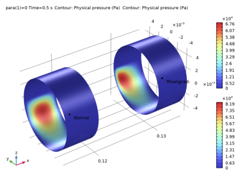
In the Settings window for 3D Plot Group, type Pressure Comparison: Right Bearing in the Label text field.
3
Locate the Data section. From the Dataset list, choose Study 1/Parametric Solutions 1 (3) (sol2).
4
From the Parameter value (para) list, choose 0.
5
Locate the Plot Settings section. Clear the Plot dataset edges check box.
6
From the View list, choose New view.
Contour 1
1
Right-click Pressure Comparison: Right Bearing and choose Contour.
2
In the Settings window for Contour, locate the Expression section.
3
In the Expression text field, type hdb.p.
4
Locate the Coloring and Style section. From the Contour type list, choose Filled.
5
From the Color table list, choose RainbowLight.
Contour 2
1
Right-click Contour 1 and choose Duplicate.
2
In the Settings window for Contour, locate the Data section.
3
From the Dataset list, choose Study 1/Parametric Solutions 1 (3) (sol2).
4
Click to expand the Inherit Style section. From the Plot list, choose Contour 1.
5
In the Model Builder window, click Results.
6
In the Settings window for Results, locate the Update of Results section.
7
Select the Only plot when requested check box.
Translation 1
1
In the Model Builder window, right-click Contour 2 and choose Translation.
2
In the Settings window for Translation, locate the Translation section.
3
In the x text field, type 3*Lb.
Pressure Comparison: Right Bearing
In the Model Builder window, under Results click Pressure Comparison: Right Bearing.
Table Annotation 1
1
In the Pressure Comparison: Right Bearing toolbar, click  More Plots and choose Table Annotation.
2
In the Settings window for Table Annotation, locate the Data section.
3
From the Source list, choose Local table.
4
Pressure Comparison: Right Bearing
1
In the Model Builder window, click Pressure Comparison: Right Bearing.
2
In the Settings window for 3D Plot Group, locate the Color Legend section.
3
From the Position list, choose Right double.
4
Click the  Zoom Extents button in the Graphics toolbar.
5
In the Pressure Comparison: Right Bearing toolbar, click  Plot.