Analyzing Porous Structures on the Microscopic Scale

Modeling flow through realistic porous structures is difficult due to the complexity of the structure itself. Resolving the flow field in detail is not feasible in real-life applications. Therefore, macroscopic approaches utilizing averaged quantities of the porous structure, such as porosity and permeability, are used. This example analyzes the flow field at the pore scale in detail. The results are used to validate and adapt the macroscopic description, which in turn are used to model large-scale porous geometries.

Model Definition

The modeled geometry shown in Figure 1 is a representative elementary volume (REV) whose properties are representative for the entire system.

Figure 1: Geometry of the REV’s pore volume.

Because only the area of the pore space is required for modeling, the porous matrix is not resolved explicitly. The REV has a quadratic cross section of 2 cm side length and a width of 6 cm. Water flows with a velocity of u = 0.1 mm/s and can flow out freely in the normal direction at the other end. The other boundaries are assumed to be symmetry boundaries. This does not correspond to the actual situation, but for modeling an REV, symmetry boundary conditions are very well suited.

To characterize the flow inside the porous structure one can estimate the Reynolds number according to

with the water density ρ = 1000 kg/m3 and viscosity μ = 10-3 Pa·s. The cross-section side length serves as the characteristic length scale, L. This results in Re = 2 and the Stokes equation can be used to describe the flow where inertia terms are neglected.

Finally, the goal of the model is to obtain the averaged values for porosity and permeability to describe a macroscopic model with, for example, Darcy’s law or the Brinkman equation. The porosity is defined as the fraction of pore space volume Vfluid to total volume Vtot:

To calculate the permeability κ (m2) the following relationship is used:

Approximating the pressure gradient ∇p by the pressure difference between the inlet and the outlet, Δp, divided by the side length L, and replacing the velocity vector u by the outlet velocity uout in the flow direction gives the expression

Results and Discussion

First of all it is interesting to have a look at the mesh, or rather the mesh quality. Although the mesh quality in itself says nothing about the quality of the results, a good mesh quality is beneficial for convergence. The overall mesh quality as shown in Figure 2 is very good.

Figure 2: Mesh quality plot.

The velocity field in the REV is shown in Figure 3. Characteristic for the flow in a porous material are areas with high and areas with low velocity. In some areas the flow also stagnates. This behavior is characterized by the permeability.

Figure 3: Velocity in the REV.

From the simulation the values for the porosity and permeability are obtained, with ε = 0.373 and

Notes About the COMSOL Implementation

An STL file of the porous structure is imported and remeshed directly in the meshing sequence. This means that the geometry sequence is kept empty. To resolve the velocity gradients at the boundaries of the porous matrix, add a boundary layer mesh.

Porous_Media_Flow_Module/Fluid_Flow/pore_scale_flow_3d

Modeling Instructions

From the menu, choose .

New

In the window, click

Model Wizard

In the window, click

In the tree, select .

Click .

Click

In the tree, select .

Click

Geometry 1

In the window, under click .

In the window for , locate the section.

From the list, choose .

Import the STL file and remesh it directly in the meshing sequence. This means that the geometry sequence will be kept empty.

Mesh 1

The meshing sequence will define the geometric model on which the physics is defined. The mesh is therefore set up completely before assigning material and physics.

Import 1

In the toolbar, click

In the window for , locate the section.

Click

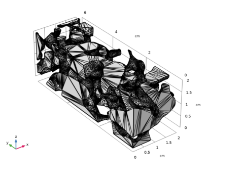
Browse to the model’s Application Libraries folder and double-click the file pore_scale_flow_3d.stl.

From the list, choose .

Increase the tolerance to collapse small and sliver mesh elements. This avoids the creation of small boundaries.

From the list, choose .

In the text field, type 1e-5.

An increased will aid the algorithm in forming as few boundaries as possible while still recognizing the planar faces.

Locate the section. In the text field, type 62.

Locate the section. Click

Join Entities 1

Join all the boundaries of the free surface to one boundary.

In the toolbar, click

Instead of clicking on boundaries in the window, paste the numbers from this document or type them in manually.

In the window for , locate the section.

Click

In the dialog box, type 14-20 in the text field.

Click .

In the window for , click

The imported STL file only contains a triangle mesh without domains. Use to form the fluid domain in the enclosed volume.

Create Domains 1

In the toolbar, click

and choose .

In the window for , click

Take a look in the log to confirm that the mesh now contains one domain and 37 boundaries.

Next, increase the quality of the triangle mesh by remeshing the faces using a operation. This will also result in triangles of more equal size.

Free Triangular 1

In the toolbar, click

and choose .

In the window for , locate the section.

From the list, choose .

Size

In the window, expand the node, then click .

In the window for , locate the section.

From the list, choose .

Free Triangular 1

Set an even finer mesh size on the free surface.

Size 1

In the window, right-click and choose .

In the window for , locate the section.

Click

In the dialog box, type 14 36 37 in the text field.

Click .

In the window for , locate the section.

Click the button.

Locate the section. Select the check box.

In the associated text field, type 0.04[cm].

Click

The surface mesh is now of good quality.

Next, generate a tetrahedral mesh in the domain of the porous structure.

Free Tetrahedral 1

In the toolbar, click

Size

In the window, expand the node, then click .

In the window for , locate the section.

From the list, choose .

Click

Boundary Layers 1

In order to resolve the large velocity gradients at the boundaries to the porous matrix properly, add a boundary layer mesh.

In the toolbar, click

Boundary Layer Properties

In the window, click .

In the window for , locate the section.

Click

In the dialog box, type 14 36 37 in the text field.

Click .

In the window for , locate the section.

In the text field, type 1.

In the text field, type 10.

Click

In the toolbar, click

Results

Mesh 1

Compare with Figure 2. The overall mesh quality is very good. The amount of mesh elements with low quality (skewness) is low. Mesh quality is not an indication for the accuracy of the solution, but it affects the convergence behavior.

Global Definitions

Add some parameters that are used to set up the model.

Parameters 1

In the window, under click .

In the window for , locate the section.

In the table, enter the following settings:


Name	Expression	Value	Description
rho_f	1000[kg/m^3]	1000 kg/m³	Fluid density
mu_f	1e-3[Pa*s]	0.001 Pa·s	Fluid viscosity
u_in	1e-4[m/s]	1E-4 m/s	Inlet velocity
width	2[cm]	0.02 m	REV width
length	6[cm]	0.06 m	REV length
V_tot	width^2*length	2.4E-5 m³	Total REV volume

Materials

Water

In the window, under right-click and choose .

In the window for , type Water in the text field.

Locate the section. In the table, enter the following settings:


Property	Variable	Value	Unit	Property group
Density	rho	rho_f	kg/m³	Basic
Dynamic viscosity	mu	mu_f	Pa·s	Basic

Creeping Flow (spf)

In the window, under click .

In the window for , click to expand the section.

From the list, choose .

Linear elements reduce the number of degrees of freedom to be solved. Because the geometry already requires a fine mesh, using linear elements decreases computational time and memory requirements while maintaining sufficient accuracy.

Inlet 1

In the toolbar, click

and choose .

Select Boundary 2 only.

In the window for , locate the section.

In the U0 text field, type u_in.

Locate the section. Click

In the dialog box, type Inlet in the text field.

Click .

Outlet 1

In the toolbar, click

and choose .

Select Boundaries 16 and 21 only.

In the window for , locate the section.

Select the check box.

Locate the section. Click

In the dialog box, type Outlet in the text field.

Click .

Create a few more selections to use them throughout the model set up.

Definitions

Wall

In the window, expand the node.

Right-click and choose .

In the window for , type Wall in the text field.

Locate the section. From the list, choose .

Select Boundaries 4, 10, and 30 only.

It might be easier to select the correct boundary by using the window. To open this window, in the toolbar click and choose . (If you are running the cross-platform desktop, you find in the main menu.)

Note that the boundary numbering differs compared to the numbering in the meshing sequence. This is due to the associativity update that runs when the Finalize node is built.

All boundaries

In the toolbar, click

In the window for , locate the section.

From the list, choose .

Select the check box.

In the text field, type All boundaries.

Symmetry

In the toolbar, click

In the window for , type Symmetry in the text field.

Locate the section. From the list, choose .

Locate the section. Under , click

In the dialog box, select in the list.

Click .

In the window for , locate the section.

Under , click

In the dialog box, in the list, choose , , and .

Click .

Creeping Flow (spf)

Symmetry 1

In the toolbar, click

and choose .

In the window for , locate the section.

From the list, choose .

Study 1

In the window, click .

In the window for , locate the section.

Clear the check box.

In the toolbar, click

Create the plot as shown in Figure 3.

In the toolbar, click

and choose .

Results

Surface 1

In the window for , locate the section.

From the list, choose .

Velocity

In the toolbar, click

In the window for , type Velocity in the text field.

Locate the section. Clear the check box.

Surface 1

Right-click and choose .

In the window for , locate the section.

From the list, choose .

Locate the section. In the text field, type 1.

Locate the section. From the list, choose .

From the list, choose .

Line 1

In the window, right-click and choose .

In the window for , locate the section.

From the list, choose .

Locate the section. From the list, choose .

From the list, choose .

In the toolbar, click

From the list, choose .

On Windows, click the colored bar underneath, or — if you are running the cross-platform desktop — the button. Choose a darker shade of gray.

Streamline 1

Right-click and choose .

In the window for , locate the section.

From the list, choose .

Locate the section. In the text field, type 40.

Locate the section. Find the subsection. From the list, choose .

Select the check box.

In the associated text field, type 0.0075.

Color Expression 1

Right-click and choose .

In the window for , locate the section.

From the list, choose .

Next, determine the porosity and permeability for our REV in order to perform simulations at the macroscopic level.

Definitions

Integration 1 (intop1)

In the toolbar, click

and choose .

In the window for , locate the section.

From the list, choose .

Average Inlet

In the toolbar, click

and choose .

In the window for , type Average Inlet in the text field.

Locate the section. From the list, choose .

From the list, choose .

Average Outlet

In the toolbar, click

and choose .

In the window for , type Average Outlet in the text field.

Locate the section. From the list, choose .

From the list, choose .

Variables 1

In the window, right-click and choose .

In the window for , locate the section.

In the table, enter the following settings:


Name	Expression	Unit	Description
por	intop1(1)/V_tot		Porosity
dPdL	-(aveop2(p)-aveop1(p))/length	N/m³	Pressure drop
u_out	spf.out1.massFlowRate/rho_f/width^2	m/s	Superficial outlet velocity
kappa	u_out*mu_f/dPdL	m²	Permeability

Since you have introduced new variables, the solution needs to be updated. It is not necessary to compute the study again.

Study 1

In the toolbar, click

Results

Global Evaluation 1

In the toolbar, click

In the window for , click in the upper-right corner of the section. From the menu, choose .

Click in the upper-right corner of the section. From the menu, choose .

Click

The results are shown in the window. The porosity is 0.371 and the permeability is about 3e-8m2. These results can now be used for calculations of large scale models.

Streamline 1

To make the results even more descriptive, create an animation.

In the window, under click .

In the window for , locate the section.

Find the subsection. From the list, choose .

In the text field, type 2000.

Animation 1

In the toolbar, click

and choose .

You can adjust the number of frames to obtain a smooth animation of the interactive arrows. This animation visualizes very nicely that there are regions in the porous medium with both very slow and very high velocity.