PDF

Estimating Permeability from Microscale Porous Structures
Introduction
This tutorial model demonstrates how to compute porosity and permeability of a sphere packing from a fully resolved microscopic model. These values are then used to model the sphere packing on the macroscopic scale using Darcy’s Law.
Model Definition
The geometry used to calculate the permeability in the microscopic scale is shown in the figure below.
Figure 1: Geometry of the unit cell of a sphere packing.
A body-centered cubic (BCC) lattice is built with spheres of two different diameters. The flow around the spheres is described using the Creeping Flow interface. A pressure difference of 1 Pa is applied between inlet (top boundary) and outlet (bottom boundary). The boundaries that correspond to the solid-fluid interface are defined as walls and the remaining boundaries are symmetry boundaries.
From this set up the porosity and permeability can be calculated. The porosity is defined as the fraction of pore space volume Vfluid to total volume Vtot
.
To calculate the permeability κ (m2) the following relationship is used
whereas the pressure gradient p is replaced by the pressure difference between inlet and outlet Δp divided by the size of the unit cell L and the velocity vector u is replaced by the outlet velocity uout in flow direction (z-direction), hence
.
The resulting values are then used to model the sphere packing on the macroscopic scale. The block height is 10 times larger than the height of the unit cell and the base area is 3 times larger.
To verify that a macroscopic approach using homogenization by deploying Darcy’s Law gives accurate values, the model compares the mass flow per unit area (L2).
Results and Discussion
The velocity field in the unit cell is shown in Figure 2.
Figure 2: Velocity in the unit cell.
From the simulation the values for the porosity and permeability are obtained, with ε = 0.49571 and .
Figure 3 shows the pressure distribution in the macroscopic model.
Figure 3: Pressure field for the macroscopic model.
The mass flow per unit area is about 0.72 kg/(m2·s) in both models.
Application Library path: Porous_Media_Flow_Module/Fluid_Flow/permeability_estimation
Modeling Instructions
From the File menu, choose New.
New
In the New window, click  Model Wizard.
Model Wizard
1
In the Model Wizard window, click  3D.
2
In the Select Physics tree, select Fluid Flow>Single-Phase Flow>Creeping Flow (spf).
3
Click Add.
4
Click  Study.
5
In the Select Study tree, select General Studies>Stationary.
6
Geometry 1
Insert the geometry sequence from a file.
1
In the Geometry toolbar, click Insert Sequence and choose Insert Sequence.
2
3
In the Geometry toolbar, click  Build All.
4
Click the  Go to Default View button in the Graphics toolbar.
Add some parameters to the Parameters list, that are used to set up the physics. The list already contains the parameters used to create the geometry and were imported automatically with the geometry sequence.
Global Definitions
Parameters 1
1
In the Model Builder window, under Global Definitions click Parameters 1.
2
In the Settings window for Parameters, locate the Parameters section.
3
Materials
Material 1 (mat1)
1
In the Model Builder window, under Component 1 (comp1) right-click Materials and choose Blank Material.
2
In the Settings window for Material, locate the Material Contents section.
3
Creeping Flow (spf)
Inlet 1
1
In the Model Builder window, under Component 1 (comp1) right-click Creeping Flow (spf) and choose Inlet.
2
In the Settings window for Inlet, locate the Boundary Condition section.
3
4
Locate the Pressure Conditions section. In the p0 text field, type p_in.
5
Outlet 1
1
In the Physics toolbar, click  Boundaries and choose Outlet.
2
Symmetry 1
1
In the Physics toolbar, click  Boundaries and choose Symmetry.
2
Use the Mass Properties to create a variable for the fluid volume and add variables that calculate porosity and permeability.
Definitions
Mass Properties 1 (mass1)
1
In the Model Builder window, under Component 1 (comp1) right-click Definitions and choose Physics Utilities>Mass Properties.
2
Variables 1
1
In the Model Builder window, right-click Definitions and choose Variables.
2
In the Settings window for Variables, locate the Variables section.
3
Mesh 1
The physics-controlled mesh sets up a boundary layer mesh at the walls which ensures a good resolution of the steep velocity gradients in that region.
In the Model Builder window, under Component 1 (comp1) right-click Mesh 1 and choose Build All.
Study 1
In the Home toolbar, click  Compute.
Results
Slice
Two default plots are created automatically. Modify the velocity plot to obtain Figure 2.
1
In the Model Builder window, expand the Velocity (spf) node, then click Slice.
2
In the Settings window for Slice, locate the Plane Data section.
3
In the Planes text field, type 1.
4
Locate the Coloring and Style section. From the Color table list, choose JupiterAuroraBorealis.
Slice 2
1
Right-click Slice and choose Duplicate.
2
In the Settings window for Slice, locate the Plane Data section.
3
From the Plane list, choose zx-planes.
4
In the Planes text field, type 1.
5
Click to expand the Inherit Style section. From the Plot list, choose Slice.
6
In the Velocity (spf) toolbar, click  Plot.
Surface 1
1
In the Model Builder window, right-click Velocity (spf) and choose Surface.
2
In the Settings window for Surface, locate the Expression section.
3
In the Expression text field, type 1.
4
Locate the Coloring and Style section. From the Coloring list, choose Uniform.
5
From the Color list, choose Gray.
Selection 1
1
Right-click Surface 1 and choose Selection.
2
In the Settings window for Selection, locate the Selection section.
3
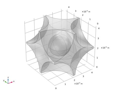
From the Selection list, choose All boundaries and remove the top, bottom and front boundaries as shown below.
Streamline 1
1
In the Model Builder window, right-click Velocity (spf) and choose Streamline.
2
3
In the Settings window for Streamline, locate the Streamline Positioning section.
4
In the Number text field, type 40.
5
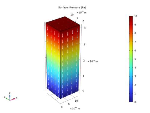
Locate the Coloring and Style section. Find the Point style subsection. From the Type list, choose Arrow.
6
Select the Number of arrows check box.
7
8
In the Velocity (spf) toolbar, click  Plot.
Color Expression 1
1
Right-click Streamline 1 and choose Color Expression.
2
In the Settings window for Color Expression, locate the Expression section.
3
In the Expression text field, type p.
4
Locate the Coloring and Style section. From the Color table list, choose GrayPrint.
Velocity (spf)
1
In the Model Builder window, under Results click Velocity (spf).
2
In the Settings window for 3D Plot Group, click to expand the Title section.
3
From the Title type list, choose None.
4
Locate the Plot Settings section. Clear the Plot dataset edges check box.
5
Locate the Color Legend section. Select the Show units check box.
6
In the Velocity (spf) toolbar, click  Plot.
Global Evaluation 1
1
In the Results toolbar, click  Global Evaluation.
2
In the Settings window for Global Evaluation, click Add Expression in the upper-right corner of the Expressions section. From the menu, choose Component 1 (comp1)>Definitions>Variables>k0 - Permeability - .
3
Click Add Expression in the upper-right corner of the Expressions section. From the menu, choose Component 1 (comp1)>Definitions>Variables>por - Porosity.
4
Click  Evaluate.
Table
1
Go to the Table window.
The permeability is about 310m2 and the porosity is 0.49571.
Root
Now, add a new component to set up a Darcy’s Law interface and use these values.
Add Component
In the Model Builder window, right-click the root node and choose Add Component>3D.
Geometry 2
Block 1 (blk1)
1
In the Geometry toolbar, click  Block.
2
In the Settings window for Block, locate the Size and Shape section.
3
In the Width text field, type 3*L.
4
In the Depth text field, type 3*L.
5
In the Height text field, type 10*L.
6
Click  Build All Objects.
Add Physics
1
In the Home toolbar, click  Add Physics to open the Add Physics window.
2
Go to the Add Physics window.
3
In the tree, select Fluid Flow>Porous Media and Subsurface Flow>Darcy’s Law (dl).
4
Find the Physics interfaces in study subsection. In the table, clear the Solve check box for Study 1.
5
Click Add to Component 2 in the window toolbar.
6
In the Home toolbar, click  Add Physics to close the Add Physics window.
Darcy’s Law (dl)
Fluid 1
1
In the Model Builder window, under Component 2 (comp2)>Darcy’s Law (dl)>Porous Medium 1 click Fluid 1.
2
In the Settings window for Fluid, locate the Fluid Properties section.
3
From the ρ list, choose User defined. In the associated text field, type rho_f.
4
From the μ list, choose User defined. In the associated text field, type mu_f.
Porous Matrix 1
1
In the Model Builder window, click Porous Matrix 1.
2
In the Settings window for Porous Matrix, locate the Matrix Properties section.
3
From the εp list, choose User defined. In the associated text field, type 0.49571.
4
From the κ list, choose User defined. In the associated text field, type 3.0292E-10.
Pressure 1
1
In the Physics toolbar, click  Boundaries and choose Pressure.
2
The macroscopic model is ten times larger in the direction of the pressure gradient than the unit cell. To compare the results of the unit cell with the results of the macroscopic model set the pressure to 10*p_in.
3
In the Settings window for Pressure, locate the Pressure section.
4
In the p0 text field, type 10*p_in.
Pressure 2
1
In the Physics toolbar, click  Boundaries and choose Pressure.
2
Add Study
1
In the Home toolbar, click  Add Study to open the Add Study window.
2
Go to the Add Study window.
3
Find the Studies subsection. In the Select Study tree, select General Studies>Stationary.
4
5
Click Add Study in the window toolbar.
6
In the Home toolbar, click  Add Study to close the Add Study window.
Study 2
1
In the Model Builder window, click Study 2.
2
In the Home toolbar, click  Compute.
Results
Again default plots are created. Modify the pressure plot to obtain Figure 3.
Arrow Surface 1
1
In the Model Builder window, right-click Pressure (dl) and choose Arrow Surface.
2
In the Settings window for Arrow Surface, click to expand the Title section.
3
From the Title type list, choose None.
4
Locate the Coloring and Style section. From the Color list, choose White.
5
In the Pressure (dl) toolbar, click  Plot.
Finally, compare the models using predefined mass flow variables. For the unit cell divide the variable by the area of the unit cell which is L^2 and not the area of the outlet boundary. For the macroscopic model use (3*L)^2. The resulting values should be almost identical.
Global Evaluation 2
1
In the Results toolbar, click  Global Evaluation.
2
In the Settings window for Global Evaluation, click Replace Expression in the upper-right corner of the Expressions section. From the menu, choose Component 1 (comp1)>Creeping Flow>Auxiliary variables>spf.out1.massFlowRate - Outward mass flow rate across feature selection - kg/s.
3
Locate the Expressions section. In the table, enter the following settings:
4
Click  Evaluate.
Global Evaluation 3
1
In the Results toolbar, click  Global Evaluation.
2
In the Settings window for Global Evaluation, locate the Data section.
3
From the Dataset list, choose Study 2/Solution 2 (3) (sol2).
4
Click Replace Expression in the upper-right corner of the Expressions section. From the menu, choose Component 2 (comp2)>Darcy’s Law>Mass flow>dl.pr2.Mflow - Mass flow - kg/s.
5
Locate the Expressions section. In the table, enter the following settings:
6
Click the Evaluate button. The results appear in the Table window.