PDF

Ion Range Benchmark
Introduction
When ions strike the surface of a solid material at extremely high energy, they may penetrate a significant distance into the target material or even pass through it. The exchange of energy between the incident ions and atoms within the target material forms the basis of a class of interactions known broadly as Single Event Effects (SEEs).
In harsh radiation environments, SEEs can cause a variety of undesirable phenomena in sensitive electronic equipment, ranging from soft errors such as bit flips to hard/permanent problems such as single event latchup or burnout. For this reason, understanding of SEEs is vital when designing electronic devices for harsh radiation environments such as outer space.
This example demonstrates an approach to modeling the interaction of energetic ions with a target material using dedicated features in the Charged Particle Tracing interface. These features are used to compute the average distance traversed by protons in silicon, which is then compared to empirical data over a range of initial energy values.
Model Definition
The Charged Particle Tracing interface includes dedicated nodes for modeling the interaction of ions with solid materials. The Particle-Matter Interaction node accounts for the energy loss and scattering of incident ions in the solid material by supporting dedicated subnodes for the following types of interactions:
The Ionization Loss subnode treats the interaction between incident ions and electrons in the target material as a continuous force that acts opposite the direction of the particle’s motion.
The Nuclear Stopping subnode treats the interaction between incident ions and nuclei in the target material as a discrete force that both slows the ion and deflects it by a random angle with a certain probability.
The validity of this approach is confirmed by this simple benchmark model. Protons are released into a block of silicon with a specified initial energy. They are then subjected to the deterministic ionization losses and stochastic nuclear interactions until their average velocity becomes negligibly small. By using an Auxiliary Dependent Variable to compute the path length of each ion in the target, the average range of the ions is computed. This average range is then compared to the tabulated range under the Continuous Slowing Down Approximation (CSDA range) as given by Ref. 1. Under the CSDA, the ions are assumed to decelerate so that rate of energy loss is the same at every point along the ion’s trajectory:
where Ei and Ef are the initial and final energy of the ion, respectively, and S(E) is the total stopping power as a function of the ion energy.
An alternative means of reporting the ion range is the projected range, which indicates the approximate penetration depth into the target material. The projected range is computed by first projecting the ion velocity onto the initial direction of propagation.
Results and Discussion
The particle trajectories are computed for initial energy values ranging from 1 keV to 100 MeV. In general, as the energy increases, the particles move in more linear trajectories as their deceleration is dominated by ionization loss. At lower initial energy values, the ion trajectories are dominated by nuclear interactions and the ions tend to move in random directions. A typical plot of the ion trajectories is shown in Figure 1.
The average ion range is reported in Figure 2 and compared to published values from Ref. 1. Both the CSDA range and the projected range are shown. As the initial ion energy increases, the agreement between the CSDA range and computed range improves because the decrease in ion energy is dominated by ionization losses, which cause the ions to decelerate continuously over time. The agreement between the CSDA range and the projected range improves as well because the ionization losses do not cause any change in the direction of ion propagation.
At lower initial energy, the CSDA range and projected range differ significantly because the ion trajectories are dominated by nuclear stopping, which causes their energy to change discontinuously and also deflects them from their initial direction of propagation. The computed path lengths then show closer agreement to the projected range than the CSDA range.
Figure 1: Trajectories of 0.1 MeV protons in silicon. The changes in direction are due to collisions with target nuclei. The continuous decrease in energy is from ionization loss.
Figure 2: Comparison of the average path length of the computed ion trajectories to the published values of the ion range. Both the CSDA range and projected range are reported.
Reference
1. NIST Stopping-Power and Range Tables for Electrons, Protons, and Helium Ions, http://www.nist.gov/pml/data/star/index.cfm
Application Library path: Particle_Tracing_Module/Charged_Particle_Tracing/ion_range_benchmark
Modeling Instructions
From the File menu, choose New.
New
In the New window, click  Model Wizard.
Model Wizard
1
In the Model Wizard window, click  3D.
2
In the Select Physics tree, select AC/DC>Particle Tracing>Charged Particle Tracing (cpt).
3
Click Add.
4
Click  Study.
5
In the Select Study tree, select General Studies>Time Dependent.
6
Load the model’s parameters.
Global Definitions
Parameters 1
1
In the Model Builder window, under Global Definitions click Parameters 1.
2
In the Settings window for Parameters, locate the Parameters section.
3
Click  Load from File.
4
Definitions
Load data for the CSDA range of protons in silicon.
Interpolation 1 (int1)
1
In the Home toolbar, click  Functions and choose Global>Interpolation.
2
In the Settings window for Interpolation, locate the Definition section.
3
From the Data source list, choose File.
4
Click  Browse.
5
6
In the Number of arguments text field, type 1.
7
Click  Import.
8
Find the Functions subsection. In the table, enter the following settings:
9
Locate the Units section. In the Argument table, enter the following settings:
10
In the Function table, enter the following settings:
Load data for the projected range of protons in silicon.
Interpolation 2 (int2)
1
In the Home toolbar, click  Functions and choose Global>Interpolation.
2
In the Settings window for Interpolation, locate the Definition section.
3
From the Data source list, choose File.
4
Click  Browse.
5
6
In the Number of arguments text field, type 1.
7
Find the Functions subsection. In the table, enter the following settings:
8
Click  Import.
9
Locate the Units section. In the Argument table, enter the following settings:
10
In the Function table, enter the following settings:
Create a block of silicon of length L centered at the origin. The value of L will be varied as a function of the particles’ initial energy E0 -- see the Parameters list.
Geometry 1
Block 1 (blk1)
1
In the Geometry toolbar, click  Block.
2
In the Settings window for Block, locate the Size and Shape section.
3
In the Width text field, type L.
4
In the Depth text field, type L.
5
In the Height text field, type L.
6
Locate the Position section. From the Base list, choose Center.
7
Click  Build All Objects.
At the maximum simulated energy of 100 MeV, the proton velocity is comparable in magnitude to the speed of light, so select the Relativistic correction option.
Charged Particle Tracing (cpt)
1
In the Model Builder window, under Component 1 (comp1) click Charged Particle Tracing (cpt).
2
In the Settings window for Charged Particle Tracing, locate the Particle Release and Propagation section.
3
Select the Relativistic correction check box.
Particle-Matter Interactions 1
1
In the Physics toolbar, click  Domains and choose Particle-Matter Interactions.
2
Ionization Loss 1
In the Physics toolbar, click  Attributes and choose Ionization Loss.
Particle-Matter Interactions 1
In the Model Builder window, click Particle-Matter Interactions 1.
Nuclear Stopping 1
In the Physics toolbar, click  Attributes and choose Nuclear Stopping.
Enter the particles’ rest mass and charge number using the variables defined in the model parameters.
Particle Properties 1
1
In the Model Builder window, under Component 1 (comp1)>Charged Particle Tracing (cpt) click Particle Properties 1.
2
In the Settings window for Particle Properties, locate the Particle Species section.
3
From the Particle species list, choose Proton.
Create a release of 1001 particles of initial energy E0 directed in the positive x direction. The particles will be released at x = L/4 in order to observe backscattered ions at low initial energies.
Release from Grid 1
1
In the Physics toolbar, click  Global and choose Release from Grid.
2
In the Settings window for Release from Grid, locate the Initial Coordinates section.
3
In the qx,0 text field, type -L/4.
4
Click  Y Range.
5
In the Range dialog box, choose Number of values from the Entry method list.
6
In the Start text field, type -L/1e3.
7
In the Stop text field, type L/1e3.
8
In the Number of values text field, type 1001.
9
Click Replace.
10
In the Settings window for Release from Grid, locate the Initial Velocity section.
11
From the Initial velocity list, choose Kinetic energy and direction.
12
In the E0 text field, type E0.
Add an auxiliary variable rp to the model. The auxiliary variable will be used to compute the total length of the particle trajectory.
Auxiliary Dependent Variable 1
1
In the Physics toolbar, click  Global and choose Auxiliary Dependent Variable.
2
In the Settings window for Auxiliary Dependent Variable, locate the Auxiliary Dependent Variable section.
3
In the R text field, type 1.
4
From the Integrate list, choose Along particle trajectory.
5
Locate the Units section. Click  Select Quantity.
6
In the Physical Quantity dialog box, type length in the text field.
7
Click  Filter.
8
In the tree, select General>Length (m).
9
Enter values for the material properties of silicon.
Materials
Material 1 (mat1)
1
In the Model Builder window, under Component 1 (comp1) right-click Materials and choose Blank Material.
2
In the Settings window for Material, locate the Material Contents section.
3
Study 1
Add a Parametric Sweep over the initial energy with a minimum value of 1 keV and a maximum value of 100 MeV.
Parametric Sweep
1
In the Study toolbar, click  Parametric Sweep.
2
In the Settings window for Parametric Sweep, locate the Study Settings section.
3
4
5
Click  Range.
6
In the Range dialog box, choose exp10(x) – Exponential function (base 10) from the Function to apply to all values list.
7
In the Start text field, type -3.
8
In the Step text field, type 1.
9
In the Stop text field, type 2.
10
Click Replace.
Step 1: Time Dependent
1
In the Model Builder window, click Step 1: Time Dependent.
2
In the Settings window for Time Dependent, locate the Study Settings section.
3
In the Output times text field, type range(0,1/20,1)*tmax.
Solution 1 (sol1)
1
In the Study toolbar, click  Show Default Solver.
Modify the default solver sequence to set a manual time step size. It is important that the time step is sufficiently small to resolve individual collisions when the ion trajectories are dominated by nuclear stopping.
2
In the Model Builder window, expand the Solution 1 (sol1) node, then click Time-Dependent Solver 1.
3
In the Settings window for Time-Dependent Solver, click to expand the Time Stepping section.
4
From the Steps taken by solver list, choose Manual.
5
In the Time step text field, type tmax/1e3.
6
In the Study toolbar, click  Compute.
Results
Particle Trajectories (cpt)
1
In the Settings window for 3D Plot Group, locate the Plot Settings section.
2
Clear the Plot dataset edges check box.
3
Locate the Data section. From the Parameter value (E0 (MeV)) list, choose 0.1.
Particle Trajectories 1
1
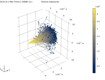
In the Model Builder window, expand the Particle Trajectories (cpt) node, then click Particle Trajectories 1.
2
In the Settings window for Particle Trajectories, locate the Coloring and Style section.
3
Find the Line style subsection. From the Type list, choose Line.
Color Expression 1
1
In the Model Builder window, expand the Particle Trajectories 1 node, then click Color Expression 1.
2
In the Settings window for Color Expression, locate the Coloring and Style section.
3
From the Color table list, choose Cividis.
4
In the Particle Trajectories (cpt) toolbar, click  Plot.
5
Click the  Go to Default View button in the Graphics toolbar. Compare the resulting plot to Figure 1.
Stopping Distance
1
In the Home toolbar, click  Add Plot Group and choose 1D Plot Group.
2
In the Settings window for 1D Plot Group, type Stopping Distance in the Label text field.
3
Locate the Data section. From the Dataset list, choose Particle 1.
4
From the Time selection list, choose Last.
5
Locate the Legend section. From the Position list, choose Upper left.
Particle 1
1
In the Stopping Distance toolbar, click  More Plots and choose Particle.
2
In the Settings window for Particle, locate the y-Axis Data section.
3
In the Expression text field, type cpt.ave(rp).
4
Locate the x-Axis Data section. From the Axis source data list, choose Outer solutions.
5
From the Parameter list, choose Expression.
6
In the Expression text field, type E0.
7
From the Unit list, choose MeV.
8
Click to expand the Coloring and Style section. Find the Line style subsection. From the Line list, choose None.
9
From the Color list, choose Red.
10
In the Width text field, type 2.
11
Find the Line markers subsection. From the Marker list, choose Star.
12
From the Positioning list, choose In data points.
Global 1
1
In the Model Builder window, right-click Stopping Distance and choose Global.
2
In the Settings window for Global, locate the y-Axis Data section.
3
4
Locate the x-Axis Data section. From the Axis source data list, choose Outer solutions.
5
From the Parameter list, choose Expression.
6
In the Expression text field, type E0.
7
From the Unit list, choose MeV.
8
Click to expand the Coloring and Style section. Find the Line style subsection. From the Line list, choose None.
9
From the Color list, choose Black.
10
Find the Line markers subsection. From the Marker list, choose Cycle.
11
From the Positioning list, choose In data points.
12
Click the  y-Axis Log Scale button in the Graphics toolbar.
13
Click the  x-Axis Log Scale button in the Graphics toolbar.
14
In the Stopping Distance toolbar, click  Plot. Compare the resulting plot to Figure 2.