PDF

Mooney-Rivlin Curve Fit
Introduction
This tutorial model demonstrates how to use the Optimization Module to estimate unknown function parameters based on measured data. The two-parameter Mooney-Rivlin solid material model is used as an example, but the procedure is generally applicable when you need to fit a parameterized analytic function to measured data.
Note: This application is also used in Introduction to the Optimization Module.
Model Definition
The two-parameter incompressible Mooney–Rivlin material model describes the local behavior of rubber-like materials. The model assumes that the local strain energy density in an incompressible solid is a simple function of local strain invariants.
In a standard tensile test, a rotationally symmetric test specimen is pulled in such a way that it extends in one direction and contracts symmetrically in the other two. For this case of uniaxial extension, the relationship between applied force, F, and resulting extension, ΔL, of a true Mooney–Rivlin material is
(1)
where A0 is the original cross-section area of the test specimen and L0 is its reference length. The constants C10 and C01 are material parameters that must be determined by fitting Equation 1 to the experimental data from the tensile test.
In practice, tensile test data is delivered in a form which is independent of the geometry of the test specimen used. There are multiple possible formats. The one used here contains corresponding measured values of engineering stress, Pi, representing force per unit reference area
and stretch, λi, representing relative elongation
The expected relationship between these variables for a Mooney–Rivlin material is
Given N pairs of measurements iPi), i = 1…, N, the values of C10 and C01 that best fit the measured data are considered to be those which minimize the total squared error
The curve-fitting problem is therefore identical to an optimization problem.
Results
Figure 1 shows measured stress and stress computed using the material properties that have been fitted to the measured data.
Figure 1: Measured (turquoise circles) and computed (blue line) engineering stresses. In addition, two other stress measures are plotted for comparison.
It should be noted that for large stretches, the values of the different stress measures will differ significantly. For a uniaxial stress state and an incompressible material like in this case, the true stress (Cauchy stress; stress per current area) is related to the engineering stress by
(2)
The 2nd Piola-Kirchhoff stress is defined as
(3)
It is thus necessary to pay attention to the stress measures actually used when a interpreting results from an actual simulation in which a material model for large stretches is used.
Application Library path: Optimization_Module/Parameter_Estimation/curve_fit_mooney_rivlin
Modeling Instructions
From the File menu, choose New.
New
In the New window, click  Blank Model.
Add Component
In the Home toolbar, click  Add Component and choose 0D.
Global Definitions
Add the stretch parameter lambda which has been varied in the measured data. Also add the unknown material parameters as global model parameters.
Parameters 1
1
In the Model Builder window, under Global Definitions click Parameters 1.
2
In the Settings window for Parameters, locate the Parameters section.
3
Variables 1
1
In the Home toolbar, click  Variables and choose Global Variables.
Set up the assumed relationship between stretch and engineering stress as a variable expression in terms of lambda and the yet unknown C10 and C01.
2
In the Settings window for Variables, locate the Variables section.
3
Add Study
1
In the Home toolbar, click  Add Study to open the Add Study window.
2
Go to the Add Study window.
3
Find the Studies subsection. In the Select Study tree, select Preset Studies for Selected Physics Interfaces>Stationary.
4
Click Add Study in the window toolbar.
5
In the Home toolbar, click  Add Study to close the Add Study window.
Use a Parameter Estimation study step to set up control variables and select an optimization solver. The Levenberg-Marquardt solver is particularly efficient for least-squares problems such as this one.
Study 1
Parameter Estimation
1
In the Study toolbar, click  Optimization and choose Parameter Estimation.
2
In the Settings window for Parameter Estimation, locate the Experimental Data section.
3
Click the Browse button. From the menu, choose Browse.
4
5
Locate the Column Settings section. In the table, click to select the cell at row number 1 and column number 2.
6
7
From the Name list, choose lambda (Stretch).
8
In the Unit text field, type 1.
9
10
In the Model expression text field, type P.
11
In the Name text field, type engStress.
12
In the Unit text field, type Pa.
13
Locate the Parameters section. Click  Add twice
14
15
Locate the Parameter Estimation Method section. From the Method list, choose Levenberg-Marquardt.
16
Find the Solver settings subsection. From the Least-squares time/parameter method list, choose From least-squares objective.
17
In the Study toolbar, click  Compute.
Results
Add a plot of the least-squares fitted stress-strain curve together with the measured data.
1D Plot Group 1
In the Home toolbar, click  Add Plot Group and choose 1D Plot Group.
Global 1
1
Right-click 1D Plot Group 1 and choose Global.
2
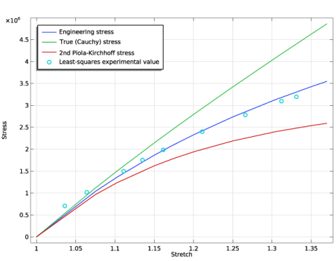
In the Settings window for Global, click Replace Expression in the upper-right corner of the y-Axis Data section. From the menu, choose Global definitions>Variables>P - Engineering stress - Pa.
3
Locate the y-Axis Data section. In the table, enter the following settings:
Global 2
1
In the Model Builder window, right-click 1D Plot Group 1 and choose Global.
2
In the Settings window for Global, click Add Expression in the upper-right corner of the y-Axis Data section. From the menu, choose Solver>Parameter estimation>opt.glsobj.engStress.data - Least-squares experimental value - Pa.
3
Click to expand the Coloring and Style section. Find the Line style subsection. From the Line list, choose None.
4
Find the Line markers subsection. From the Marker list, choose Circle.
5
From the Positioning list, choose In data points.
6
In the 1D Plot Group 1 toolbar, click  Plot.
1D Plot Group 1
Finish the plot by adjusting the title, axis labels, and legend positioning.
1
In the Model Builder window, click 1D Plot Group 1.
2
In the Settings window for 1D Plot Group, click to expand the Title section.
3
From the Title type list, choose None.
4
Locate the Plot Settings section. Select the x-axis label check box.
5
6
Select the y-axis label check box.
7
8
Locate the Legend section. From the Position list, choose Upper left.
Evaluation Group 1
In the Results toolbar, click  Evaluation Group.
1D Plot Group 1
Click the  Zoom Extents button in the Graphics toolbar.
Global Evaluation 1
In the Model Builder window, right-click Evaluation Group 1 and choose Global Evaluation.
Evaluation Group 1
1
In the Settings window for Evaluation Group, locate the Data section.
2
From the Parameter selection (lambda) list, choose Last.
Global Evaluation 1
Use the predefined Objective value node to evaluate the estimated values of material parameters C01 and C10.
1
In the Model Builder window, click Global Evaluation 1.
2
In the Settings window for Global Evaluation, click Add Expression in the upper-right corner of the Expressions section. From the menu, choose Solver>Control parameters>C10 - Mooney-Rivlin parameter - Pa.
3
Click Add Expression in the upper-right corner of the Expressions section. From the menu, choose Solver>Control parameters>C01 - Mooney-Rivlin parameter - Pa.
4
In the Evaluation Group 1 toolbar, click  Evaluate.