PDF

Temperature-Dependent Plasticity in Pressure Vessel
Introduction
This example demonstrates how to use temperature dependent materials within the Nonlinear Structural Materials Module. Material data such as Young’s modulus, yield stress and strain hardening have strong temperature dependencies.
A large container holds pressurized hot water. Several pipes are attached to the pressure vessel. Those pipes can rapidly transfer cold water in case of an emergency cooling. The pressure vessel is made of carbon steel with an internal cladding of stainless steel. In case of a fast temperature transient, the differences in thermal expansion properties between the materials cause high stresses.
Model Definition
Geometry
The pressure vessel has the shape of a closed cylinder. Four pipes are attached at two levels along its height. At each level, the pipes are equidistantly spaced around the container.
The pipes are welded into the vessel and the welding can be considered as a chamfer between those two parts. The structure, together with its key dimensions, is presented in Figure 1.
Figure 1: Pressure vessel and the dimensions for the vessel-pipe connection.
The structure has the following dimensions:
Inner vessel radius, rv = 1000 mm,
Inner pipe radius, rp = 60 mm,
Vessel thickness, tv = 100 mm,
Pipe thickness, tp = 40 mm.
The vessel length, lv, and the pipe length, lp, are large compared to the thickness of both parts. For modeling purposes, they need to be large enough so that local effects at the vessel-pipe connection can be disregarded. The chamfer extends 20 mm from the corner at the connection between the pipe and the vessel.
The dual material consists of a thin 10 mm layer of stainless steel (dark gray in Figure 1) that faces the water, and carbon steel (light gray in Figure 1) that faces the outside air.
In order to save computational time, only the connection between one pipe and the vessel is modeled, as shown on the left image of Figure 1.
Material Model
The thermoelastic material data of stainless steel is given in Table 1. Table 2 shows the yield stress as a function of plastic strain at temperatures of 20, 100, 200, and 300 °C.
α (1/°C)
cp (J/(kg·K))
σys(0.0) (MPa)
σys(0.0004) (MPa)
σys(0.001) (MPa)
σys(0.002) (MPa)
σys(0.004) (MPa)
σys(0.001) (MPa)
The yield stress of the carbon steel is two or three times higher than that of stainless steel. It is therefore considered as elastic. Its material properties are shown in Table 3.
α (1/°C)
cp (J/(kg·K))
The heat transfer coefficient between steel and air is 10 W/(m2·K), and between steel and water it is 100 W/(m2·K).
Boundary conditions
A pressure of 70 bar acts on the inner walls of the vessel and the pipe. The temperature on the inside of the pressure vessel is initially at 280 °C, while the outside air remains at 50 °C. Suddenly and instantaneously, cold water at 20 °C is pumped through the pipe into the vessel, where the hot water needs 30 minutes to cool down to 20 °C. The cooling speed is constant.
Model Assumptions
Due to symmetries, only a 45° sector of the vessel is modeled. The influence of the hot water pressure at the end of the vessel is approximated with an axial stress of 33.3 MPa, which is 4.76 times the inner pressure. The parameters lv and lp are both set to 200 mm.
Results and Discussion
Three studies are performed in this analysis. In an initial step, the mechanical and thermal stationary state is computed. This serves as initial conditions for a transient step which solves the heat transfer problem only, where the cold water flows through the pipe, cooling the initially hot water in the vessel. A comparison of the temperature profiles, before and after the event, are shown in Figure 2. After 30 min, the water inside the vessel has cooled down to 20 °C, but the container is still locally more than 100 °C warmer. This leads to large gradients in the thermal strains.
Figure 2: Temperature profiles before and after the cooling event.
The last step solves the elastoplastic deformation with temperature-dependent material parameters. The development of plastic strains in the stainless steel layer is shown in Figure 3. From the figure it can be seen that a plastic zone develops as the vessel cools down. Initially, when the vessel is at steady state, some plastic strains are generated by stresses caused by differences in the thermal expansion of the two steels. In a real structure, such stresses would have been relaxed after the first service cycle. In the transient study, when the vessel cools down and the yield limit increases, the pipe deforms plastically in other locations.
Figure 3: Plastic strains before and after the cooling event.
As the temperature decreases, the yield stress increases, so warm parts are more sensitive to high stresses. Figure 4 shows the von Mises stress after 30 min of cooling.
Figure 4: Distribution of von Mises stress after cooling down the hot water.
Figure 5 shows the membrane plus bending stress intensity distribution during the cooling. It is clear that the location of the maximum intensity changes along the time. At the end of the cooling the maximum remains close to the nozzle.
Figure 5: Membrane plus bending stress intensity at initial time (top), 1140 s (middle), and 1800 s (bottom).
Figure 6 shows the maximum of the membrane plus bending stress intensity variation during the cooling. One noticed there is a minimum around 1140 s.
Figure 6: Maximum of membrane plus bending stress intensity with time.
Figure 7 shows the computed and linearized stress at initial time (solid) and once the cooling is done (dotted line).
Figure 7: Computed stress (blue), Membrane stress (green), and Membrane plus bending stress (red) at initial time(solid line) and finale time (dotted line).
Notes About the COMSOL Implementation
COMSOL Multiphysics can handle material data depending on several parameters. Use Interpolation functions, which you can select from the Definitions or Materials nodes. You can type in the data in a table or define your function in a text file. Use the symbol % in a text file to include comments or headers.
In this example, the Young’s modulus E(T), coefficient of thermal expansion α(T), thermal conductivity k(T), and heat capacity at constant pressure Cp(T) are defined in the Materials node from interpolated data. The initial yield stress σy0(T) and the nonlinear hardening function σh(T, εpe) are defined by data imported from a text file.
Interpolation functions can handle any number of arguments. For convenience, specify units (Pa, m, s, and so on) for the function and arguments. When applicable, COMSOL Multiphysics automatically scales any input into the correct unit. For more details see the section Operators, Functions, and Constants in the COMSOL Multiphysics Reference Manual.
In this example there are two cuts that are “almost symmetry cuts” in the sense that they should stay plane but are still allowed to move in the normal direction. One is the cut in the pipe, and the other is the cut through the pressure vessel wall. In order to accomplish this, a Symmetry node is used, but with free displacement as a normal direction condition. Thus the normal direction displacement is constant, but yet determined by the solution. The Symmetry node has different flavors of normal direction constraints, where the default is equivalent to a traditional symmetry condition.
Heat transfer in solids is a time-dependent phenomenon, and since plasticity is a path-dependent process, it is important to capture the evolution of temperature profiles accurately. You need to limit the time step in the BDF solver settings to account for the rate at which thermal loads change in time. Use a different study step to compute the elastoplastic deformation after computing the heat transfer. Since this is not a coupled problem, this segregated approach reduces computational time.
Application Library path: Nonlinear_Structural_Materials_Module/Plasticity/temperature_dependent_plasticity
Modeling Instructions
From the File menu, choose New.
New
In the New window, click  Model Wizard.
Model Wizard
1
In the Model Wizard window, click  3D.
2
In the Select Physics tree, select Structural Mechanics>Thermal-Structure Interaction>Thermal Stress, Solid.
3
Click Add.
4
Click  Study.
5
In the Select Study tree, select General Studies>Stationary.
6
Global Definitions
Parameters 1
1
In the Model Builder window, under Global Definitions click Parameters 1.
2
In the Settings window for Parameters, locate the Parameters section.
3
The thermal shock caused by the cold water is time dependent. Therefore the variable for time, t, needs to be set to zero so that the heat boundary conditions can be evaluated also in the static analysis.
Geometry 1
1
In the Geometry toolbar, click Insert Sequence and choose Insert Sequence.
2
3
In the Geometry toolbar, click  Build All.
4
Click the  Go to Default View button in the Graphics toolbar.
Full geometry instructions can be found in Appendix — Geometry Modeling Instructions.
Solid Mechanics (solid)
Linear Elastic Material 1
In the Model Builder window, under Component 1 (comp1)>Solid Mechanics (solid) click Linear Elastic Material 1.
Plasticity 1
1
In the Physics toolbar, click  Attributes and choose Plasticity.
2
3
In the Settings window for Plasticity, locate the Plasticity Model section.
4
Find the Isotropic hardening model subsection. From the list, choose Hardening function.
Materials
Stainless Steel
1
In the Model Builder window, under Component 1 (comp1) right-click Materials and choose Blank Material.
2
In the Settings window for Material, type Stainless Steel in the Label text field.
3
4
Locate the Material Contents section. In the table, enter the following settings:
Add Young’s modulus as a function of temperature for the stainless steel.
Interpolation 1 (int1)
1
In the Model Builder window, expand the Component 1 (comp1)>Materials>Stainless Steel (mat1) node.
2
Right-click Component 1 (comp1)>Materials>Stainless Steel (mat1)>Young’s modulus and Poisson’s ratio (Enu) and choose Functions>Interpolation.
3
In the Settings window for Interpolation, locate the Definition section.
4
In the Function name text field, type fE.
5
6
Locate the Units section. In the Argument table, enter the following settings:
7
In the Function table, enter the following settings:
Stainless Steel (mat1)
Add the temperature as a model input for the Young’s modulus property.
1
In the Model Builder window, under Component 1 (comp1)>Materials>Stainless Steel (mat1) click Young’s modulus and Poisson’s ratio (Enu).
2
In the Settings window for Young’s Modulus and Poisson’s Ratio, locate the Model Inputs section.
3
Click  Select Quantity.
4
In the Physical Quantity dialog box, type temperature in the text field.
5
Click  Filter.
6
In the tree, select General>Temperature (K).
7
8
In the Settings window for Young’s Modulus and Poisson’s Ratio, locate the Output Properties section.
9
Add the coefficient of thermal expansion as a function of temperature for the stainless steel.
Interpolation 1 (int1)
1
In the Home toolbar, click  Functions and choose Global>Interpolation.
2
In the Settings window for Interpolation, locate the Definition section.
3
In the Function name text field, type fA.
4
5
Locate the Units section. In the Argument table, enter the following settings:
6
In the Function table, enter the following settings:
Add the thermal conductivity as a function of temperature for the stainless steel.
Interpolation 2 (int2)
1
In the Home toolbar, click  Functions and choose Global>Interpolation.
2
In the Settings window for Interpolation, locate the Definition section.
3
In the Function name text field, type fK.
4
5
Locate the Units section. In the Argument table, enter the following settings:
6
In the Function table, enter the following settings:
Add the heat capacity as a function of temperature for the stainless steel.
Interpolation 3 (int3)
1
In the Home toolbar, click  Functions and choose Global>Interpolation.
2
In the Settings window for Interpolation, locate the Definition section.
3
In the Function name text field, type fCp.
4
5
Locate the Units section. In the Argument table, enter the following settings:
6
In the Function table, enter the following settings:
Stainless Steel (mat1)
Add the temperature as a model input for the Basic properties.
1
In the Model Builder window, under Component 1 (comp1)>Materials>Stainless Steel (mat1) click Basic (def).
2
In the Settings window for Basic, locate the Model Inputs section.
3
Click  Select Quantity.
4
In the Physical Quantity dialog box, click  Filter.
5
In the tree, select General>Temperature (K).
6
7
In the Model Builder window, click Stainless Steel (mat1).
8
In the Settings window for Material, locate the Material Contents section.
9
10
Locate the Material Properties section. In the Material properties tree, select Solid Mechanics>Elastoplastic Material>Elastoplastic Material Model.
11
Click  Add to Material.
Load the table containing yield stress as function of plastic strain and temperature.
Interpolation 1 (int1)
1
In the Home toolbar, click  Functions and choose Global>Interpolation.
2
In the Settings window for Interpolation, locate the Definition section.
3
From the Data source list, choose File.
4
Click  Browse.
5
6
Find the Functions subsection. In the table, enter the following settings:
7
Locate the Units section. In the Argument table, enter the following settings:
8
In the Function table, enter the following settings:
9
Locate the Definition section. Click  Import.
Stainless Steel (mat1)
Add the temperature and the equivalent plastic strain as model inputs for the Elastoplastic material model properties.
1
In the Model Builder window, under Component 1 (comp1)>Materials>Stainless Steel (mat1) click Elastoplastic material model (ElastoplasticModel).
2
In the Settings window for Elastoplastic Material Model, locate the Model Inputs section.
3
Click  Select Quantity.
4
In the Physical Quantity dialog box, click  Filter.
5
In the tree, select General>Temperature (K).
6
7
In the Settings window for Elastoplastic Material Model, locate the Model Inputs section.
8
Click  Select Quantity.
9
In the Physical Quantity dialog box, type plastic strain in the text field.
10
Click  Filter.
11
In the tree, select Solid Mechanics>Equivalent plastic strain (1).
12
13
In the Settings window for Elastoplastic Material Model, locate the Output Properties section.
14
The hardening function is the stress increase from the initial yield stress. As the full stress-strain curve is given, subtract the stress at zero equivalent plastic strain.
Carbon Steel
1
In the Model Builder window, right-click Materials and choose Blank Material.
2
In the Settings window for Material, type Carbon Steel in the Label text field.
3
4
Locate the Material Contents section. In the table, enter the following settings:
Add Young’s modulus as function of temperature for the carbon steel.
Interpolation 1 (int1)
1
In the Model Builder window, expand the Component 1 (comp1)>Materials>Carbon Steel (mat2) node.
2
Right-click Component 1 (comp1)>Materials>Carbon Steel (mat2)>Young’s modulus and Poisson’s ratio (Enu) and choose Functions>Interpolation.
3
In the Settings window for Interpolation, locate the Definition section.
4
In the Function name text field, type fE.
5
6
Locate the Units section. In the Argument table, enter the following settings:
7
In the Function table, enter the following settings:
Add the temperature as a model input for the Young’s modulus property.
Carbon Steel (mat2)
1
In the Model Builder window, under Component 1 (comp1)>Materials>Carbon Steel (mat2) click Young’s modulus and Poisson’s ratio (Enu).
2
In the Settings window for Young’s Modulus and Poisson’s Ratio, locate the Model Inputs section.
3
Click  Select Quantity.
4
In the Physical Quantity dialog box, type temperature in the text field.
5
Click  Filter.
6
In the tree, select General>Temperature (K).
7
Add the coefficient of thermal expansion as function of temperature for the carbon steel.
Interpolation 1 (int1)
1
In the Home toolbar, click  Functions and choose Global>Interpolation.
2
In the Settings window for Interpolation, locate the Definition section.
3
In the Function name text field, type fA.
4
5
Locate the Units section. In the Argument table, enter the following settings:
6
In the Function table, enter the following settings:
Interpolation 2 (int2)
1
In the Home toolbar, click  Functions and choose Global>Interpolation.
Add the thermal conductivity as function of temperature for the carbon steel.
2
In the Settings window for Interpolation, locate the Definition section.
3
In the Function name text field, type fK.
4
5
Locate the Units section. In the Argument table, enter the following settings:
6
In the Function table, enter the following settings:
Add the heat capacity as function of temperature for the carbon steel.
Interpolation 3 (int3)
1
In the Home toolbar, click  Functions and choose Global>Interpolation.
2
In the Settings window for Interpolation, locate the Definition section.
3
In the Function name text field, type fCp.
4
5
Locate the Units section. In the Argument table, enter the following settings:
6
In the Function table, enter the following settings:
Carbon Steel (mat2)
Add the temperature as a model input for the Basic properties.
1
In the Model Builder window, under Component 1 (comp1)>Materials>Carbon Steel (mat2) click Basic (def).
2
In the Settings window for Basic, locate the Model Inputs section.
3
Click  Select Quantity.
4
In the Physical Quantity dialog box, click OK.
5
In the Model Builder window, click Carbon Steel (mat2).
6
In the Settings window for Material, locate the Material Contents section.
7
Definitions
Add the time history for the temperature of the water in the pipe.
Step 1 (step1)
1
In the Home toolbar, click  Functions and choose Local>Step.
2
In the Settings window for Step, type pipeWaterTemp in the Function name text field.
3
Locate the Parameters section. In the Location text field, type 1.
4
In the From text field, type 280.
5
In the To text field, type 20.
Add the time history for the temperature of the water in the pressure vessel.
Interpolation 1 (int1)
1
In the Home toolbar, click  Functions and choose Local>Interpolation.
2
In the Settings window for Interpolation, locate the Definition section.
3
In the Function name text field, type vesselWaterTemp.
4
5
Locate the Units section. In the Argument table, enter the following settings:
6
In the Function table, enter the following settings:
Create an explicit selection to use in the symmetry boundary conditions.
Symmetry Boundaries
1
In the Definitions toolbar, click  Explicit.
2
In the Settings window for Explicit, type Symmetry Boundaries in the Label text field.
3
Locate the Input Entities section. From the Geometric entity level list, choose Boundary.
4
Heat Transfer in Solids (ht)
Initial Values 1
1
In the Model Builder window, under Component 1 (comp1)>Heat Transfer in Solids (ht) click Initial Values 1.
2
In the Settings window for Initial Values, locate the Initial Values section.
3
In the T text field, type 280[degC].
Symmetry 1
1
In the Physics toolbar, click  Boundaries and choose Symmetry.
2
In the Settings window for Symmetry, locate the Boundary Selection section.
3
From the Selection list, choose Symmetry Boundaries.
Heat Flux 1
1
In the Physics toolbar, click  Boundaries and choose Heat Flux.
2
3
In the Settings window for Heat Flux, locate the Heat Flux section.
4
From the Flux type list, choose Convective heat flux.
5
In the h text field, type 10.
6
In the Text text field, type 50[degC].
Heat Flux 2
1
In the Physics toolbar, click  Boundaries and choose Heat Flux.
2
3
In the Settings window for Heat Flux, locate the Heat Flux section.
4
From the Flux type list, choose Convective heat flux.
5
In the h text field, type 100.
6
In the Text text field, type pipeWaterTemp(t[1/s])[degC].
Heat Flux 3
1
In the Physics toolbar, click  Boundaries and choose Heat Flux.
2
3
In the Settings window for Heat Flux, locate the Heat Flux section.
4
From the Flux type list, choose Convective heat flux.
5
In the h text field, type 100.
6
In the Text text field, type vesselWaterTemp(t).
Solid Mechanics (solid)
In the Model Builder window, under Component 1 (comp1) click Solid Mechanics (solid).
Symmetry 1
1
In the Physics toolbar, click  Boundaries and choose Symmetry.
2
In the Settings window for Symmetry, locate the Boundary Selection section.
3
From the Selection list, choose Symmetry Boundaries.
You will overwrite the extra boundaries of the explicit selection with a another Symmetry node, but with free displacement as normal constraint.
Symmetry 2
1
In the Physics toolbar, click  Boundaries and choose Symmetry.
2
3
In the Settings window for Symmetry, click to expand the Normal Direction Condition section.
4
From the list, choose Free displacement.
Symmetry 3
1
In the Physics toolbar, click  Boundaries and choose Symmetry.
2
3
In the Settings window for Symmetry, locate the Normal Direction Condition section.
4
From the list, choose Free displacement.
Boundary Load 1
1
In the Physics toolbar, click  Boundaries and choose Boundary Load.
2
3
In the Settings window for Boundary Load, locate the Force section.
4
From the Load type list, choose Pressure.
5
In the p text field, type internalPressure.
Boundary Load 2
1
In the Physics toolbar, click  Boundaries and choose Boundary Load.
2
3
In the Settings window for Boundary Load, locate the Force section.
4
Specify the FA vector as
You will now add a Stress Linearization node to compute the linearized stress in the vessel.
Stress Linearization 1
1
In the Physics toolbar, click  Global and choose Stress Linearization.
2
In the Settings window for Stress Linearization, locate the Linearization section.
3
From the Type list, choose Distributed.
Using the Distributed type, you can find the critical location. You can later on set the starting point of the stress linearization line.
4
Locate the Boundary Selection section. Click to select the  Activate Selection toggle button.
5
6
Locate the Domain Selection section. Click to select the  Activate Selection toggle button.
7
Mesh 1
Free Quad 1
1
In the Mesh toolbar, click  Boundary and choose Free Quad.
2
Size 1
1
Right-click Free Quad 1 and choose Size.
2
In the Settings window for Size, locate the Element Size section.
3
Click the Custom button.
4
Locate the Element Size Parameters section. Select the Maximum element size check box.
5
Swept 1
1
In the Mesh toolbar, click  Swept.
2
In the Settings window for Swept, locate the Domain Selection section.
3
From the Geometric entity level list, choose Domain.
4
Distribution 1
1
In the Model Builder window, right-click Swept 1 and choose Distribution.
2
In the Settings window for Distribution, locate the Distribution section.
3
In the Number of elements text field, type 5.
Free Quad 2
1
In the Mesh toolbar, click  Boundary and choose Free Quad.
2
Size 1
1
Right-click Free Quad 2 and choose Size.
2
In the Settings window for Size, locate the Element Size section.
3
Click the Custom button.
4
Locate the Element Size Parameters section. Select the Maximum element size check box.
5
Swept 2
1
In the Mesh toolbar, click  Swept.
2
In the Settings window for Swept, locate the Domain Selection section.
3
From the Geometric entity level list, choose Domain.
4
Distribution 1
1
Right-click Swept 2 and choose Distribution.
2
In the Settings window for Distribution, locate the Distribution section.
3
From the Distribution type list, choose Predefined.
4
In the Element ratio text field, type 3.
5
Select the Reverse direction check box.
Swept 3
1
In the Mesh toolbar, click  Swept.
2
In the Settings window for Swept, locate the Domain Selection section.
3
From the Geometric entity level list, choose Domain.
4
Distribution 1
1
Right-click Swept 3 and choose Distribution.
2
In the Settings window for Distribution, locate the Distribution section.
3
In the Number of elements text field, type 2.
Swept 4
In the Mesh toolbar, click  Swept.
Distribution 1
1
Right-click Swept 4 and choose Distribution.
2
In the Settings window for Distribution, locate the Distribution section.
3
In the Number of elements text field, type 2.
4
Click  Build Selected.
Study 1: Initialization
1
In the Model Builder window, click Study 1.
2
In the Settings window for Study, type Study 1: Initialization in the Label text field.
In an initialization study, the mechanical and the thermal stationary state is computed. This serves as initial conditions for a transient step.
3
In the Home toolbar, click  Compute.
Add Study
1
In the Home toolbar, click  Add Study to open the Add Study window.
In a second study, the transient temperature distribution is computed.
2
Go to the Add Study window.
3
Find the Studies subsection. In the Select Study tree, select General Studies>Time Dependent.
4
Find the Physics interfaces in study subsection. In the table, clear the Solve check box for Solid Mechanics (solid).
5
Click Add Study in the window toolbar.
Study 2
Step 1: Time Dependent
1
In the Settings window for Time Dependent, locate the Study Settings section.
2
In the Output times text field, type range(0,0.2,2) range(60,60,1800).
Analyze half an hour, storing the results once every minute. The first steps are refined in order to improve the convergence.
3
Click to expand the Values of Dependent Variables section. Find the Initial values of variables solved for subsection. From the Settings list, choose User controlled.
4
From the Method list, choose Solution.
5
From the Study list, choose Study 1: Initialization, Stationary.
6
Find the Values of variables not solved for subsection. From the Settings list, choose User controlled.
7
From the Method list, choose Solution.
8
From the Study list, choose Study 1: Initialization, Stationary.
9
In the Model Builder window, click Study 2.
10
In the Settings window for Study, type Study 2: Heat Transfer in the Label text field.
11
Locate the Study Settings section. Clear the Generate default plots check box.
Solution 2 (sol2)
1
In the Study toolbar, click  Show Default Solver.
2
In the Model Builder window, expand the Solution 2 (sol2) node, then click Time-Dependent Solver 1.
3
In the Settings window for Time-Dependent Solver, click to expand the Time Stepping section.
Since cold water is suddenly injected in the vessel, it is important to capture the development accurately, so you want to enforce intermediate steps.
4
From the Steps taken by solver list, choose Intermediate.
5
In the Study toolbar, click  Compute.
Add Study
1
Go to the Add Study window.
2
Find the Studies subsection. In the Select Study tree, select General Studies>Stationary.
3
Find the Physics interfaces in study subsection. In the table, clear the Solve check box for Heat Transfer in Solids (ht).
4
Click Add Study in the window toolbar.
In a third study, the elastoplastic problem is computed using a stationary continuation study step.
5
In the Study toolbar, click  Add Study to close the Add Study window.
Study 3
Step 1: Stationary
1
In the Settings window for Stationary, click to expand the Values of Dependent Variables section.
2
Find the Initial values of variables solved for subsection. From the Settings list, choose User controlled.
3
From the Method list, choose Solution.
4
From the Study list, choose Study 1: Initialization, Stationary.
5
Find the Values of variables not solved for subsection. From the Settings list, choose User controlled.
6
From the Method list, choose Solution.
7
From the Study list, choose Study 2: Heat Transfer, Time Dependent.
8
From the Time (s) list, choose Automatic (all solutions).
9
Click to expand the Study Extensions section. Select the Auxiliary sweep check box.
10
11
12
In the Model Builder window, click Study 3.
13
In the Settings window for Study, type Study 3: Plasticity in the Label text field.
14
Locate the Study Settings section. Clear the Generate default plots check box.
Solution 3 (sol3)
1
In the Study toolbar, click  Show Default Solver.
2
In the Model Builder window, expand the Solution 3 (sol3) node.
3
In the Model Builder window, expand the Study 3: Plasticity>Solver Configurations>Solution 3 (sol3)>Stationary Solver 1 node, then click Fully Coupled 1.
4
In the Settings window for Fully Coupled, click to expand the Method and Termination section.
Use a double dogleg solver in order to improve the convergence.
5
From the Nonlinear method list, choose Double dogleg.
6
In the Study toolbar, click  Compute.
Results
Volume 1
1
In the Model Builder window, expand the Stress (solid) node, then click Volume 1.
2
In the Settings window for Volume, locate the Expression section.
3
From the Unit list, choose MPa.
Stress (solid)
1
In the Model Builder window, click Stress (solid).
2
In the Settings window for 3D Plot Group, locate the Data section.
3
From the Dataset list, choose Study 3: Plasticity/Solution 3 (sol3).
Deformation
1
In the Model Builder window, under Results>Stress (solid)>Volume 1 click Deformation.
2
In the Settings window for Deformation, locate the Scale section.
3
Select the Scale factor check box.
4
5
In the Stress (solid) toolbar, click  Plot.
Equivalent Plastic Strain (solid)
1
In the Model Builder window, under Results click Equivalent Plastic Strain (solid).
2
In the Settings window for 3D Plot Group, locate the Data section.
3
From the Dataset list, choose Study 3: Plasticity/Solution 3 (sol3).
4
In the Equivalent Plastic Strain (solid) toolbar, click  Plot.
5
From the Parameter value (t (s)) list, choose 0.
6
In the Equivalent Plastic Strain (solid) toolbar, click  Plot.
7
From the Parameter value (t (s)) list, choose 1200.
8
In the Equivalent Plastic Strain (solid) toolbar, click  Plot.
Temperature (ht)
1
In the Model Builder window, click Temperature (ht).
2
In the Settings window for 3D Plot Group, locate the Data section.
3
From the Dataset list, choose Study 3: Plasticity/Solution 3 (sol3).
Surface
1
In the Model Builder window, expand the Temperature (ht) node, then click Surface.
2
In the Settings window for Surface, locate the Expression section.
3
From the Unit list, choose degC.
4
In the Temperature (ht) toolbar, click  Plot.
Temperature (ht)
1
In the Model Builder window, click Temperature (ht).
2
In the Settings window for 3D Plot Group, locate the Data section.
3
From the Parameter value (t (s)) list, choose 0.
4
In the Temperature (ht) toolbar, click  Plot.
In the steps below you will investigate the bending and membrane stress in the vessel. First evaluate the maximum of the stress intensity for all time steps.
Stress Intensity, Maximum
1
In the Results toolbar, click  Evaluation Group.
2
In the Settings window for Evaluation Group, type Stress Intensity, Maximum in the Label text field.
3
Locate the Data section. From the Dataset list, choose Study 3: Plasticity/Solution 3 (sol3).
Surface Maximum 1
1
Right-click Stress Intensity, Maximum and choose Maximum>Surface Maximum.
2
3
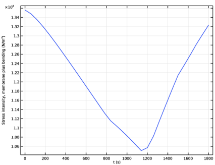
In the Settings window for Surface Maximum, click Replace Expression in the upper-right corner of the Expressions section. From the menu, choose Component 1 (comp1)>Solid Mechanics>Stress linearization>solid.SImb - Stress intensity, membrane plus bending - N/m².
4
Click to expand the Configuration section. Select the Include position check box.
5
In the Stress Intensity, Maximum toolbar, click  Evaluate.
The evaluation of the stress intensity over the whole surface for all time steps can take few minutes.
Table
1
Go to the Table window.
2
Click Table Graph in the window toolbar.
Results
Stress Intensity, Maximum
1
In the Model Builder window, under Results click 1D Plot Group 7.
2
In the Settings window for 1D Plot Group, type Stress Intensity, Maximum in the Label text field.
Table Graph 1
1
In the Model Builder window, expand the Stress Intensity, Maximum node, then click Table Graph 1.
2
In the Settings window for Table Graph, locate the Data section.
3
From the Plot columns list, choose Manual.
4
In the Columns list, select Stress intensity, membrane plus bending (N/m^2).
5
In the Stress Intensity, Maximum toolbar, click  Plot.
The plot shows that the maximum of stress intensity has a dip just before 1200s. Let’s look at the distribution of the stress intensity at different time: start, end, and at the dip.
Stress Intensity
1
In the Home toolbar, click  Add Plot Group and choose 3D Plot Group.
2
In the Settings window for 3D Plot Group, type Stress Intensity in the Label text field.
3
Locate the Data section. From the Dataset list, choose Study 3: Plasticity/Solution 3 (sol3).
Surface 1
Right-click Stress Intensity and choose Surface.
Selection 1
1
In the Model Builder window, right-click Surface 1 and choose Selection.
2
Surface 1
1
In the Model Builder window, click Surface 1.
2
In the Settings window for Surface, click Replace Expression in the upper-right corner of the Expression section. From the menu, choose Component 1 (comp1)>Solid Mechanics>Stress linearization>solid.SImb - Stress intensity, membrane plus bending - N/m².
Marker 1
1
Right-click Surface 1 and choose Marker.
2
In the Settings window for Marker, locate the Display section.
3
From the Display list, choose Max.
4
In the Stress Intensity toolbar, click  Plot.
Stress Intensity
1
In the Model Builder window, under Results click Stress Intensity.
2
In the Settings window for 3D Plot Group, locate the Data section.
3
From the Parameter value (t (s)) list, choose 1140.
4
In the Stress Intensity toolbar, click  Plot.
5
From the Parameter value (t (s)) list, choose 0.
6
In the Stress Intensity toolbar, click  Plot.
You will now plot the stress linearization line at the critical location.
Linearization Line
1
In the Model Builder window, expand the Results>Datasets node, then click Linearization Line.
2
In the Settings window for Cut Line 3D, locate the Data section.
3
From the Dataset list, choose Study 3: Plasticity/Solution 3 (sol3).
Stress Linearization (sl1)
1
In the Model Builder window, under Results click Stress Linearization (sl1).
2
In the Settings window for 1D Plot Group, locate the Data section.
3
From the Time selection list, choose From list.
4
In the Parameter values (t (s)) list, choose 0 and 1800.
Stress Tensor, Linearization Line System
1
In the Model Builder window, expand the Stress Linearization (sl1) node, then click Stress Tensor, Linearization Line System.
2
In the Settings window for Line Graph, click to expand the Coloring and Style section.
3
In the Width text field, type 2.
4
Click to expand the Legends section. In the Legend text field, type Computed [eval(t) s].
Membrane Stress
1
In the Model Builder window, click Membrane Stress.
2
In the Settings window for Line Graph, locate the Coloring and Style section.
3
In the Width text field, type 2.
4
Locate the Legends section. In the Legend text field, type Membrane [eval(t) s].
Membrane Plus Bending Stress
1
In the Model Builder window, click Membrane Plus Bending Stress.
2
In the Settings window for Line Graph, locate the Coloring and Style section.
3
In the Width text field, type 2.
4
Locate the Legends section. In the Legend text field, type Membrane + Bending [eval(t) s].
Solid Mechanics (solid)
Stress Linearization 1
1
In the Model Builder window, under Component 1 (comp1)>Solid Mechanics (solid) click Stress Linearization 1.
2
In the Settings window for Stress Linearization, click to expand the Postprocessing section.
In the Stress Intensity Maximum evaluation group you can find the coordinates of the critical point.
3
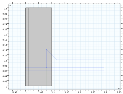
Specify the Linearization line, starting point vector as
Study 3: Plasticity
Solution 3 (sol3)
In the Model Builder window, under Study 3: Plasticity>Solver Configurations right-click Solution 3 (sol3) and choose Solution>Update.
Results
Stress Linearization (sl1)
1
In the Settings window for 1D Plot Group, locate the Legend section.
2
From the Position list, choose Lower left.
3
In the Stress Linearization (sl1) toolbar, click  Plot.
 
Appendix — Geometry Modeling Instructions
From the File menu, choose New.
New
In the New window, click  Model Wizard.
Model Wizard
1
In the Model Wizard window, click  3D.
2
In the Select Physics tree, select Structural Mechanics>Thermal-Structure Interaction>Thermal Stress, Solid.
3
Click Add.
4
Click  Study.
5
In the Select Study tree, select General Studies>Stationary.
6
Geometry 1
Work Plane 1 (wp1)
1
In the Geometry toolbar, click  Work Plane.
2
In the Settings window for Work Plane, locate the Plane Definition section.
3
From the Plane list, choose xz-plane.
4
Locate the Unite Objects section. Clear the Unite objects check box.
5
Click  Show Work Plane.
Work Plane 1 (wp1)>Polygon 1 (pol1)
1
In the Work Plane toolbar, click  Polygon.
2
In the Settings window for Polygon, locate the Coordinates section.
3
From the Data source list, choose Vectors.
4
In the xw text field, type 1.3 1.08 1.08 1.08 1.08 1.12 1.12 1.3 1.3 1.3.
5
In the yw text field, type 0.07 0.07 0.07 0.14 0.14 0.1 0.1 0.1 0.1 0.07.
6
Click  Build Selected.
Work Plane 1 (wp1)>Rectangle 1 (r1)
1
In the Work Plane toolbar, click  Rectangle.
2
In the Settings window for Rectangle, locate the Size and Shape section.
3
In the Width text field, type 0.3.
4
In the Height text field, type 0.01.
5
Locate the Position section. In the xw text field, type 1.
6
In the yw text field, type 0.06.
7
Click  Build Selected.
Revolve 1 (rev1)
1
In the Model Builder window, under Component 1 (comp1)>Geometry 1 right-click Work Plane 1 (wp1) and choose Revolve.
2
In the Settings window for Revolve, locate the Revolution Axis section.
3
Find the Direction of revolution axis subsection. In the xw text field, type 1.
4
In the yw text field, type 0.
5
Locate the Revolution Angles section. Click the Angles button.
6
In the End angle text field, type -90.
7
Click  Build Selected.
Work Plane 2 (wp2)
1
In the Geometry toolbar, click  Work Plane.
2
In the Settings window for Work Plane, locate the Plane Definition section.
3
From the Plane list, choose xz-plane.
4
Locate the Unite Objects section. Clear the Unite objects check box.
5
Click  Show Work Plane.
Work Plane 2 (wp2)>Rectangle 1 (r1)
1
In the Work Plane toolbar, click  Rectangle.
2
In the Settings window for Rectangle, locate the Size and Shape section.
3
In the Width text field, type 0.09.
4
In the Height text field, type 0.3.
5
Locate the Position section. In the xw text field, type 1.01.
6
Click  Build Selected.
Work Plane 2 (wp2)>Rectangle 2 (r2)
1
In the Work Plane toolbar, click  Rectangle.
2
In the Settings window for Rectangle, locate the Size and Shape section.
3
In the Width text field, type 0.01.
4
In the Height text field, type 0.3.
5
Locate the Position section. In the xw text field, type 1.
6
Click  Build Selected.
Revolve 2 (rev2)
1
In the Model Builder window, under Component 1 (comp1)>Geometry 1 right-click Work Plane 2 (wp2) and choose Revolve.
2
In the Settings window for Revolve, locate the Revolution Angles section.
3
Click the Angles button.
4
In the End angle text field, type 45.
5
Click  Build Selected.
6
Click the  Zoom Extents button in the Graphics toolbar.
Difference 1 (dif1)
1
In the Geometry toolbar, click  Booleans and Partitions and choose Difference.
2
In the Settings window for Difference, locate the Difference section.
3
Select the Keep objects to subtract check box.
4
Clear the Keep interior boundaries check box.
5
Select the object rev1(2) only.
6
Find the Objects to subtract subsection. Click to select the  Activate Selection toggle button.
7
Select the object rev2(2) only.
8
Click  Build Selected.
Difference 2 (dif2)
1
In the Geometry toolbar, click  Booleans and Partitions and choose Difference.
2
In the Settings window for Difference, locate the Difference section.
3
Select the Keep objects to subtract check box.
4
Select the object rev1(1) only.
5
Find the Objects to subtract subsection. Click to select the  Activate Selection toggle button.
6
Select the object rev2(1) only.
7
Click  Build Selected.
Cylinder 1 (cyl1)
1
In the Geometry toolbar, click  Cylinder.
2
In the Settings window for Cylinder, locate the Size and Shape section.
3
In the Radius text field, type 0.06.
4
In the Height text field, type 0.4.
5
Locate the Position section. In the x text field, type 0.95.
6
Locate the Axis section. From the Axis type list, choose Cartesian.
7
In the x text field, type 1.
8
In the z text field, type 0.
9
Click  Build Selected.
Difference 3 (dif3)
1
In the Geometry toolbar, click  Booleans and Partitions and choose Difference.
2
Select the objects rev2(1) and rev2(2) only.
3
In the Settings window for Difference, locate the Difference section.
4
Find the Objects to subtract subsection. Click to select the  Activate Selection toggle button.
5
6
Click  Build Selected.
Difference 4 (dif4)
1
In the Geometry toolbar, click  Booleans and Partitions and choose Difference.
2
3
In the Settings window for Difference, locate the Difference section.
4
Find the Objects to subtract subsection. Click to select the  Activate Selection toggle button.
5
6
Select the Keep objects to subtract check box.
7
Click  Build Selected.
8
In the Geometry toolbar, click  Build All.