PDF

STL Import 2 —
Remeshing an Imported Mesh1
Introduction
The STL file format is one of the standard file formats for 3D printing, and it is also often used as a format for exchanging 3D scan data. STL files contain only the triangulated surface, which we can also call a surface mesh, of a 3D object. The triangles in the file are identified by their normals and vertex coordinates which together form a faceted representation of the object.
COMSOL Multiphysics supports import of an STL file both as a surface mesh and as a geometry with smooth faces. This tutorial series focuses on using available tools to edit imported surface meshes, the different ways of repairing the meshes, and how to generate a volume mesh from the imported surface mesh, either directly or by first creating a geometry with smooth faces from the mesh. Regardless of which method you choose to follow, COMSOL Multiphysics supports a variety of operations, for example:
There are certain things to consider when choosing whether to create a geometry or not. Working with the mesh directly can be more robust in case you need to intersect several imported meshes (or intersect the imported mesh with geometric objects of more complex shapes). It is recommended that you create a geometry if your steps to prepare the imported mesh for simulation involve using a Swept mesh operation to generate a structured mesh.
This tutorial, the second in the series, demonstrates a workflow where a simulation mesh is generated by remeshing the imported surface mesh, without creating a geometry. The steps from importing the STL file to creating the final mesh are described in detail and include repairing of the imported mesh, combining the imported mesh with a mesh generated to represent a surrounding volume, intersecting the mesh with a plane, remeshing, creating domains, generating the tetrahedral mesh, and finally visualizing the mesh elements using a mesh plot.
STL Import 1 — Generating a Geometry from an Imported Mesh, the first part of this tutorial series, describes the process of creating a geometry from an imported STL file.
The two tutorials in this series are complementary, and intend to provide a detailed insight into how to work with imported meshes. Apart from arriving at a simulation mesh in two different ways, the tutorials also cover repairing different types of defects, and different ways of visualizing the mesh. Depending on your application and the imported mesh at hand, pick and choose from the tools detailed in the tutorials to arrive at a mesh that suits your needs.
Lastly, it is important to mention that the techniques used in the tutorial series apply to any type of imported surface meshes, such as the formats PLY and 3MF. They also apply when creating a mesh from a Filter or Partition dataset, which you would do when using the results of a simulation as the mesh for a new simulation, for example during a topology optimization study.
Model Definition
Import the STL file of a vertebra geometry shown below.
Follow the instructions in this tutorial to
Application Library path: COMSOL_Multiphysics/Meshing_Tutorials/stl_vertebra_mesh_import
Modeling Instructions
From the File menu, choose New.
New
In the New window, click  Model Wizard.
Model Wizard
1
In the Model Wizard window, click  3D.
2
Geometry 1
1
In the Model Builder window, under Component 1 (comp1) click Geometry 1.
2
In the Settings window for Geometry, locate the Units section.
3
From the Length unit list, choose mm.
This will set the same length unit also for the mesh.
Mesh 1
Import 1
1
In the Mesh toolbar, click  Import.
2
In the Settings window for Import, locate the Import section.
3
Click  Browse.
4
5
From the Boundary partitioning list, choose Minimal.
This setting is suitable when importing mesh files that have no obvious boundary partitioning, for example meshes generated by medical imaging techniques. After the import, the mesh will usually consist of only one boundary that you can partition as needed, using the available tools. Use the Automatic or Detect boundaries settings when importing meshes that contain planar faces and fillets, which can then be detected to partition the mesh accordingly.
6
Click  Import.
Transform 1
You can easily move, rotate, and scale an imported mesh by adding a Transform subnode to an Import node. Add several Transform subnodes to rotate an imported mesh around more than one axis. Here, we will move the mesh to the origin.
1
In the Mesh toolbar, click  More Attributes and choose Transform.
2
In the Settings window for Transform, locate the Displacement section.
3
In the x text field, type -10[mm].
4
In the y text field, type -90[mm].
5
In the z text field, type -10[mm].
6
Click  Build Selected.
Create Domains 1
1
In the Mesh toolbar, click  Create Entities and choose Create Domains.
This operation is needed before you can generate a tetrahedral mesh. It checks if the imported surface mesh forms any watertight regions, and if so, it forms domains.
2
In the Settings window for Create Domains, click  Build Selected.
Warning
A warning appears stating that the operation failed to create a domain for the face of the vertebra.
1
In the Model Builder window, click Warning.
2
Expand the Warning node and click on the Warning subnode for more details.
Warning
This Warning indicates that the mesh of the vertebra does not form a watertight component. The edges that appear in the selection for the Warning node are exterior edges that are adjacent to one or several holes in the mesh. Disable the rendering of the mesh to see them more clearly in the Graphics window.
1
Click the  Mesh Rendering button in the Graphics toolbar. Zoom in to see the exact view below.
There are three holes, which are all located on the same side of the vertebra. You can verify this by going through the list of edges or by turning on Wireframe Rendering to make sure there are no other edges hiding behind the faces of the vertebra. If you do, remember to turn off Wireframe Rendering before continuing.
The larger hole in the bottom left is a triangular hole that seems to be caused by a missing mesh element. The two additional holes located on the upper half of the image are both slit like holes that have zero or almost zero area, as we will see soon when we zoom in on the individual holes. Such slits usually result when the vertices of the imported mesh triangles do not match within the specified import tolerance.
We will use two techniques to repair the holes as they require different kind of treatment. Of the three holes in the image above, first we will repair the one in the upper right corner of the image, we will continue with the small hole in the upper left. Lastly, fill in the triangular hole in the bottom left.
2
From the Windows menu, choose Selection List.
If there are more than 3 edges listed in the Selection List, go back to the Import 1 node and make sure that the setting Boundary partitioning is set to Minimal, then reimport the mesh.
Keep the Selection List open as you will use it throughout the tutorial.
Selection List
1
Go to the Selection List window.
2
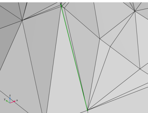
In the list, select 3 (selected, meshed) (the edge located in the upper right corner of the previous image).
3
Click the  Zoom to Selection button in the Graphics toolbar.
4
Click the  Mesh Rendering button in the Graphics toolbar.
The selected edge is next to a very narrow slit that has the same number of edge elements on both sides. Zoom in further at the upper center of the image above, a bit down from the end of the slit where the shorter edge elements are located.
The corners of the triangular elements do not match, since the corresponding mesh vertices were not merged during the import. To fix this, reimport the file using a larger tolerance.
Mesh 1
Import 1
1
In the Model Builder window, expand the Warning node, then click Component 1 (comp1)>Mesh 1>Import 1.
2
In the Settings window for Import, locate the Import section.
3
From the Repair tolerance list, choose Absolute.
4
In the Absolute tolerance text field, type 1e-4[mm].
5
Click  Import.
The mesh vertices are now merged, thereby eliminating the hole and the edge adjacent to it. You can easily verify this by hovering over the location of the hole with the pointer: no edge becomes highlighted.
Next, repair the other slit in the mesh.
Selection List
1
Go to the Selection List window.
2
3
Click the  Zoom to Selection button in the Graphics toolbar.
4
On one side of the slit (on the left side of the red edge in the figure) there is one triangle element, whereas on the other side there are two elements. Since the import functionality cannot partition elements or add new elements, the mesh edges on the two sides of the slit could not be merged even with the larger tolerance. To repair the slit, we will use the Fill Holes operation, which can introduce new mesh edges in order to merge edges. The Fill Holes operation searches for holes within a selection of boundaries and will automatically fill all holes that are smaller than a specified tolerance. We can therefore use this operation to also repair the third hole.
Mesh 1
Fill Holes 1
1
In the Mesh toolbar, click  Create Entities and choose Fill Holes.
In the Model Builder window, note that the Fill Holes 1 node is inserted after the Import 1 node in the model tree, since the Import 1 was the current node. The current node is indicated by a frame around its icon, either green (node is built) or yellow (node is not built). It is desired to insert operations that fix the holes before creating a domain, so leave the Create Domains 1 node unbuilt for now.
2
3
In the Settings window for Fill Holes, click  Build Selected.
The slit has been repaired by introducing a mesh edge on the left side of the slit, merging the two sides of the hole, and removing the edge. Now, let’s find out if the third hole is also repaired.
4
Click the  Mesh Rendering button in the Graphics toolbar.
5
Click the  Go to Default View button in the Graphics toolbar, to check if any edges remain. You can zoom in a bit to see the exact view as in the image below.
The original triangular hole (bottom left corner in the above image) remains since it is larger than the automatically determined tolerance for Fill Holes. Measure the perimeter of the remaining hole to obtain an estimate for the tolerance value to use with the Fill Holes feature.
6
In the Graphics window toolbar, clicknext to  Select Boundaries, then choose Select Edges.
7
8
In the Mesh toolbar, click  Measure.
The length of the edge is reported in the Messages window. It is about 2.2 mm long.
9
Go back to the Settings window for Fill Holes.
10
Locate the Fill Holes section. From the Fill holes tolerance list, choose Manual.
11
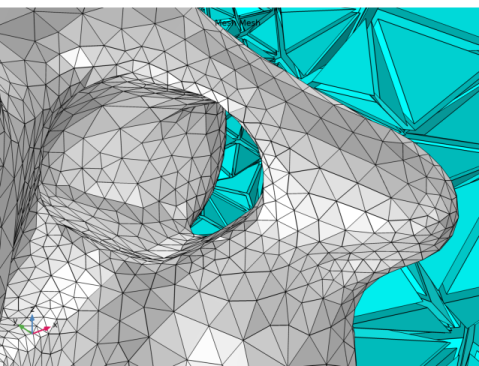
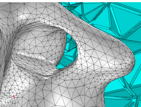
In the Maximum hole perimeter text field, type 2.3[mm]. The value you enter here should be slightly larger than the measured hole perimeter.
12
Click  Build Selected.
This concludes the repair of the imported mesh, which now forms a watertight boundary. Continue with the steps below to learn how to combine the imported mesh with a block created in the same component, how to intersect the mesh with a plane to delete a portion of the mesh, and generate a volume mesh both inside and outside the vertebra. The mesh of the block could just as well be imported from file, if available.
Geometry 1
Block 1 (blk1)
1
In the Geometry toolbar, click  Block.
Choose the size and position of the block such that it will contain the vertebra mesh.
2
In the Settings window for Block, locate the Size and Shape section.
3
In the Width text field, type 30[mm].
4
In the Depth text field, type 20[mm].
5
In the Height text field, type 25[mm].
6
Locate the Position section. From the Base list, choose Center.
7
Click  Build Selected.
8
Click the  Go to Default View button in the Graphics toolbar.
Mesh 2
A second mesh (Mesh 2) was automatically added when the block was added to the geometry sequence. Mesh 2 is conforming with Geometry 1 while Mesh 1 defines its own geometric model with its own set of entities (domains, boundaries, edges, and points). The frame around the Mesh 1 icon indicates that any physics that you will add to the Component will be defined on Mesh 1. In the Settings window for the Component 1 node, you can easily switch so that the physics will be defined on Geometry 1 instead. There is no need for that here as we are interested in analyzing the vertebra.
Continue to generate a mesh for the block using default mesh size settings.
Size
1
In the Model Builder window, expand the Component 1 (comp1)>Meshes node.
2
Right-click Component 1 (comp1)>Meshes>Mesh 2 and choose Build All.
This will automatically add a Free Tetrahedral operation to Mesh 2 as the block is a solid object.
3
Click the  Mesh Rendering button in the Graphics toolbar.
Mesh 1
Import 2
1
In the Model Builder window, expand the Component 1 (comp1)>Meshes>Mesh 1 node.
2
Right-click Mesh 1 and choose Import. Make sure the Import 2 node is added after Fill Holes 1 in the model tree.
3
In the Settings window for Import, locate the Import section.
4
From the Source list, choose Meshing sequence. This will automatically suggest to import Mesh 2, which is the mesh of the block.
5
Clear the Import domain elements check box.
You only need to import the surface mesh for the block to the meshing sequence of the vertebra, as overlapping volume elements are not supported.
6
Click Import.
7
Click the  Transparency button in the Graphics toolbar, to see the vertebra inside the block.
8
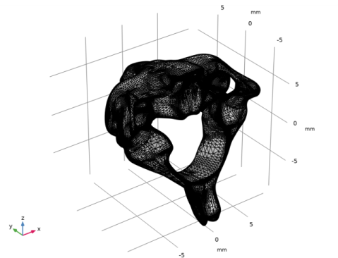
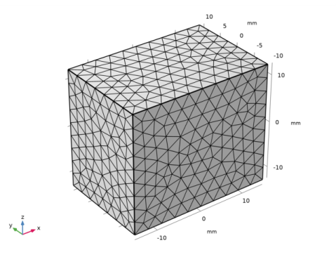
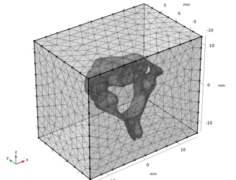
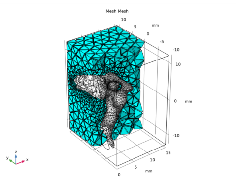
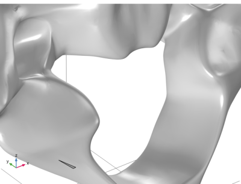
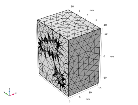
Rotate the mesh in the Graphics window to check that the vertebra is fully contained in the block, the two meshes should not intersect.
You can also use mesh Statistics to check that only triangle elements were imported for the block.
9
In the Model Builder window, right-click Mesh 1 and select Statistics.
The mesh should not contain any domain elements. This means that the first part of the Statistics section should only list Triangles, Edge elements, and Vertex elements. If tetrahedra are present, or if the meshes intersect, check and make sure that the settings for Block 1 and Import 2 are correct, then reimport the mesh of the block.
In the Statistics window, we can also see that the Minimum element quality of the surface mesh is rather low (about 1.7e-4). Furthermore, the Element quality histogram reveals that a large portion of the elements have low quality. You will remesh the vertebra further ahead to get a higher element quality.
As both boundary meshes are imported and do not contain any holes, build the Create Domains 1 node.
Create Domains 1
1
In the Model Builder window, right-click Create Domains 1 and choose Build Selected.
2
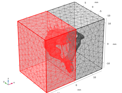
Check the Messages window. Two domains were created; one for the vertebra and one for the domain of the surrounding block.
Continue with intersecting the mesh of the block and vertebra with an assumed symmetry plane.
Intersect with Plane 1
1
In the Mesh toolbar, click  Booleans and Partitions and choose Intersect with Plane.
2
In the Settings window for Intersect with Plane, locate the Plane Definition section.
3
From the Plane list, choose yz-plane.
4
Locate the Cleanup section. From the Repair tolerance list, choose Absolute.
The Absolute tolerance is set to 0.01 mm by default, which is the value we will use here. The Automatic setting uses a higher tolerance (0.09 mm).
5
Click  Build Selected.
You should now be able to see in the Graphics window that the mesh of the vertebra and the block have been partitioned by the plane. A new mesh face that connects the vertebra and the block along the plane has also been created inside the block. This is controlled by the Create intersection faces check box. When it is selected, the operation creates planar faces inside closed edge loops generated by the intersection.
Intersecting a mesh can introduce small and sliver mesh elements. The cleanup part of the operation collapses these, but in doing so, it may change the shape of the mesh that is intersected to ensure a planar intersection face. A lower tolerance will preserve the original shape of the mesh better, but will also keep more of the small and sliver elements introduced by the intersection. Here, the lower tolerance helps to better keep the original shape and avoid some small faces. The small faces result when parts of the vertebra that are very close to the intersecting plane are collapsed onto the plane.
Delete Entities 1
In the Mesh toolbar, click  Delete Entities.
Selection List
1
Go to the Selection List window.
2
3
Click Add to Selection in the window toolbar.
Mesh 1
Delete Entities 1
1
In the Model Builder window, click Delete Entities 1.
2
In the Settings window for Delete Entities, click  Build Selected to delete the part of the vertebra and block on one side of the symmetry plane.
3
Click the  Go to Default View button in the Graphics toolbar.
4
In the Graphics window toolbar, clicknext to  Select Domains, then choose Select Boundaries.
5
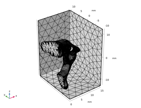
In the Selection list, confirm that you have the expected nine boundaries; six for the block and three for the vertebra. If there are more than nine boundaries in the list, check the tolerance setting for the Intersect with plane operation.
After intersecting a mesh with a plane, remeshing is usually needed to eliminate small elements that often result from the intersection. Also, the mesh on intersection faces is always generated as coarsely as possible, and will typically need to be refined. Remeshing the faces will result in mesh elements of more uniform size, and will also result in triangles that are closer to the wanted equilateral shape.
6
Click the  Transparency button in the Graphics toolbar, as this makes it easier to see the mesh on the outside of the block. Also, if you have turned off Mesh Rendering earlier, turn it on again.
7
In the Model Builder window, click Mesh 1.
8
Click the  Click and Hide button in the Graphics toolbar.
9
10
Click the  Click and Hide button in the Graphics toolbar again to deactivate the functionality and avoid hiding more boundaries.
Next, you will remesh the faces with the Free Triangular operation to generate a finer mesh and improve element quality. This may be needed when the quality of an imported mesh is not suitable for the simulation at hand or, as discussed earlier, to improve the mesh on the intersection faces and close to the intersection edges.
Free Triangular 1
1
In the Mesh toolbar, click  Boundary and choose Free Triangular.
2
Select Boundaries 2–9 only. This is most easily done from the Selection List, as some of the boundaries are hidden.
The mesh on the far end of the block (Boundary 1) has not been modified, and is of good quality. Therefore, there is no need to remesh it.
3
In the Settings window for Free Triangular, click to expand the Mesh Preprocessing section.
4
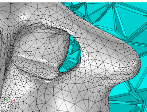
In the Relative simplification tolerance text field, type 0.001. The lowered tolerance allows for a closer representation of the curved parts of the vertebra faces with smaller radius.
Size 1
1
In the Model Builder window, right-click Free Triangular 1 and choose Size.
This adds a size attribute, Size 1, to the Free Triangular operation. Use it to set a smaller element size on the boundary of the vertebra. The first subnode specifies the default element size for the operation, which applies to all boundaries, unless it is overridden by other size settings.
2
In the Settings window for Size, locate the Geometric Entity Selection section.
3
Click  Clear Selection.
4
5
Locate the Element Size section. From the Predefined list, choose Fine.
It is possible to change the individual mesh size parameters to customize the mesh size even further. This is described in the meshing tutorial Adjusting the Element Size for the Unstructured Mesh Generator, available in the Application Libraries.
6
Click  Build Selected.
The mesh now consists of approximately 6500 triangles.
When generating a new mesh with the Free Triangular operation, smooth surfaces are first created in the background, based on the original mesh. These surfaces are then used when the new mesh is generated. See the discussion in the section Comparing the Meshed Geometry with the STL Mesh in the tutorial STL Import 1 Generating a Geometry from an Imported Mesh for more information on how the Relative simplification tolerance influences the shape of the faces to remesh.
Another alternative is to modify the mesh using the Adapt operation with an absolute size expression. For an imported linear mesh, the software creates a smooth surface in the background, which is used to place new or moved mesh vertices when adapting the mesh.
7
On the Mesh toolbar, click the Statistics button.
In the Messages window, you can verify that the Minimum element quality is now much improved (0.32) and the high average quality (0.80) indicates that most of the triangle elements have a good quality.
Now, fill the domains with a volume mesh.
Free Tetrahedral 1
1
In the Mesh toolbar, click  Free Tetrahedral.
2
In the Settings window for Free Tetrahedral, click  Build Selected.
The Messages window reports that the two domains contain about 53 000 domain elements. If you check the Selection List window, you can also see that the two domains listed there are marked as ’(meshed)’ and that there are no unmeshed domains left. This means that the mesh is now ready and can be used to set up materials and physics for a 3D simulation in the software.
Before concluding the tutorial, let’s take a closer look at how to create and customize a mesh plot for a visual inspection of the mesh.
3
In the Mesh toolbar, click  Plot.
The default mesh plot shows the quality of the mesh elements. The light green color indicates a good quality mesh (quality close to 1).
Results
Mesh 1
Follow the steps below to create a plot of the volume elements colored according to the domain they belong to, and filtering applied to see the elements inside the block and vertebra.
1
In the Settings window for Mesh, locate the Coloring and Style section.
2
From the Element color list, choose White to color the mesh elements white.
3
Click to expand the Element Filter section. Select the Enable filter check box.
4
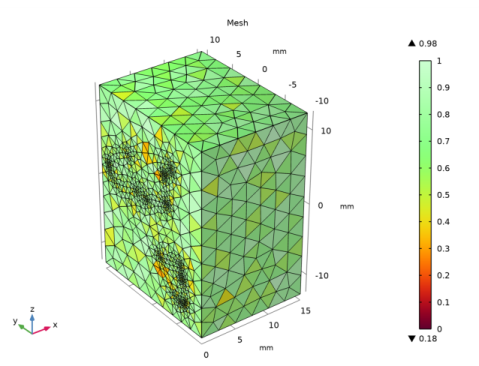
In the Expression text field, type x>1[mm] to visualize elements with at least one vertex with x-coordinate higher than 1 mm.
5
In the Mesh Plot 1 toolbar, click  Plot.
Next, add a Selection to the plot node and select the vertebra domain.
Selection 1
1
Right-click Mesh 1 and choose Selection.
2
3
In the Mesh Plot 1 toolbar, click  Plot.
Now, duplicate the Mesh 1 plot node and make some changes to color the surrounding elements in a light blue color.
Mesh 2
Right-click Mesh 1 and choose Duplicate.
Selection 1
1
In the Model Builder window, expand the Mesh 2 node, then click Selection 1.
2
In the Settings window for Selection, locate the Selection section.
3
Click  Clear Selection.
4
Mesh 2
1
In the Model Builder window, click Mesh 2.
2
In the Settings window for Mesh, locate the Coloring and Style section.
3
From the Element color list, choose Cyan.
4
Locate the Element Filter section. In the Expression text field, type y>1[mm].
5
Click to expand the Shrink Elements section. In the Element scale factor text field, type 0.8.
6
In the Mesh Plot 1 toolbar, click  Plot.
Set the Element scale factor to a value smaller than 1 to inspect how individual mesh elements are connected, as you can then see the parts of the surrounding elements that would otherwise be hidden behind the first layer of elements in the view. You can enter a value larger than 1 to increase the size of the elements in the plot. Use this when you need to inspect the shape of individual elements that are really small.
When the mesh conforms with a geometry in the model, the elements are curved to match the boundaries of the geometry, according to the specified geometry shape function. If there is no geometry, as is the case for imported meshes, the curved elements are generated in one of two ways: For imported linear elements, as this STL file of the vertebra, the software estimates the shape of surfaces and curves from the linear elements to place higher-order nodes. Else, for mesh files that contain second-order elements, as some NASTRAN and COMSOL Multiphysics files do, the software extracts this information to curve the boundary elements and place higher-order nodes accordingly. A curved, second-order representation of the geometry shape is automatically used when solving for most physics interfaces. On the other hand, CFD problems are typically solved using a linear geometry shape function.
Follow the remaining few steps to visualize the curved elements and higher-order nodes on the boundary of the vertebra.
Mesh Plot 1
1
In the Model Builder window, click Mesh Plot 1.
2
In the Settings window for 3D Plot Group, locate the Plot Settings section.
3
Clear the Plot dataset edges check box.
4
In the Mesh Plot 1 toolbar, click  Plot to hide the black edges of the block and vertebra. You can turn them on again later if you want to see them.
5
This is what the mesh looks like with a linear representation of the faces. Now, change the Geometry shape function to plot second-order elements.
Mesh 1
1
In the Model Builder window, expand the Results>Datasets node, then click Mesh 1.
2
In the Settings window for Mesh, locate the Mesh section.
3
From the Geometry shape function list, choose Quadratic Lagrange.
Note that this is just a plot setting and does not influence the Geometry shape function used when solving.
Mesh 1
1
In the Model Builder window, under Results>Mesh Plot 1 click Mesh 1.
2
The faces are now represented with second-order elements which results in a smoother shape.
Lastly, let’s add the node points of the second-order elements to the plot.
3
In the Settings window for Mesh, locate the Coloring and Style section.
4
From the Node points list, choose Geometry shape function.
5
In the Mesh Plot 1 toolbar, click  Plot.
 

1
The STL geometry is provided courtesy of Mark Yeoman, Continuum Blue, UK.