PDF

STL Import 1 —
Generating a Geometry from an Imported Mesh1
Introduction
The STL file format is one of the standard file formats for 3D printing, and it is also often used as a format for exchanging 3D scan data. STL files contain only the triangulated surface, which we can also call a surface mesh, of a 3D object. The triangles in the file are identified by their normals and vertex coordinates which together form a faceted representation of the object.
COMSOL Multiphysics supports import of an STL file both as a surface mesh and as a geometry with smooth faces. This tutorial series focuses on using available tools to edit imported surface meshes, the different ways of repairing the meshes, and how to generate a volume mesh from the imported surface mesh, either directly or by first creating a geometry with smooth faces from the mesh. Regardless of which method you choose to follow, COMSOL Multiphysics supports a variety of operations, for example:
There are certain things to consider when choosing whether to create a geometry or not. Working with the mesh directly can be more robust in case you need to intersect several imported meshes (or intersect the imported mesh with geometric objects of more complex shapes). It is recommended that you create a geometry if your steps to prepare the imported mesh for simulation involve using a Swept mesh operation to generate a structured mesh.
STL Import 2 — Remeshing an Imported Mesh, the second part of this tutorial series, describes the process of preparing a mesh directly by remeshing it, without creating a geometry.
The two tutorials in this series are complementary, and intend to provide a detailed insight into how to work with imported meshes. Apart from arriving at a simulation mesh in two different ways, the tutorials also cover repairing different types of defects, and different ways of visualizing the mesh. Depending on your application and the imported mesh at hand, pick and choose from the tools detailed in the tutorials to arrive at a mesh that suits your needs.
Lastly, it is important to mention that the techniques used in the tutorial series apply to any type of imported surface meshes, such as the formats PLY and 3MF. They also apply when creating a mesh from a Filter or Partition dataset, which you would do when using the results of a simulation as the mesh for a new simulation, for example during a topology optimization study.
Model Definition
Import the STL file of a vertebra geometry shown below.
Follow the instructions in this tutorial to
Application Library path: COMSOL_Multiphysics/Meshing_Tutorials/stl_vertebra_import
Modeling Instructions
From the File menu, choose New.
New
In the New window, click  Model Wizard.
Model Wizard
1
In the Model Wizard window, click  3D.
2
Geometry 1
Import 1 (imp1)
1
In the Home toolbar, click  Import.
2
In the Settings window for Import, locate the Import section.
3
Click  Browse.
4
5
Click  Import.
The import of an STL file consists of three steps: the import of the surface mesh from the file, the generation of a surface geometry from the imported mesh, and finally the creation of a solid object. After the import is complete the geometry appears on the screen.
Notice that after the import completes, the reference to the STL file is no longer visible in the Settings window. The source for the geometry import is now Mesh Part 1, which is where the mesh import can be found. The Mesh Part 1 sequence is added under the Global Definitions>Mesh Parts node. The output of a mesh import sequence added here can be imported into any geometry sequence in the mph file. The Import 1 node in the geometry sequence handles the last steps of the process: conversion from mesh to geometry and creation of a solid object.
According to the information in the Messages window, a mixed object was generated by the import. This means that the object contains both solids and surfaces. Some parts of the STL source mesh form a "watertight" shell that can be converted into a solid. The additional faces are not needed in this case, so these must be found and deleted.
6
Click  Go to Source to locate the source mesh in the Model Builder window.
Mesh Part 1
The mesh import automatically partitions the STL mesh into boundaries based on, for example, an angle criteria. By inspecting the boundaries, it is possible to find mesh faces that are not properly connected to others. Do this by opening the Selection List window, clicking on each of the boundaries in the list, and checking in the Graphics window if the boundary is wanted or not.
1
From the Windows menu, choose Selection List.
2
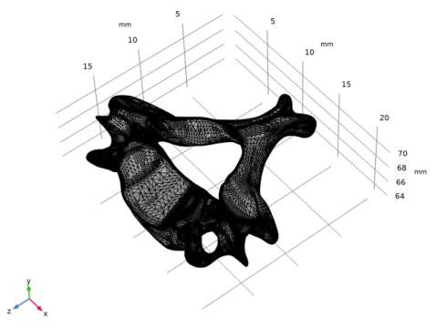
In the Model Builder window, expand the Global Definitions>Mesh Parts>Mesh Part 1 node, then click Mesh Part 1.
3
In the Graphics window toolbar, clicknext to  Select Domains, then choose Select Boundaries.
If there are many boundaries, reimport the mesh with the import setting Boundary partitioning: Minimal as this will partition the mesh into as few boundaries as possible. If reimporting the mesh takes a long time, use the Join operation to join the boundaries manually, as shown below.
Join Entities 1
1
In the Mesh toolbar, click  Join Entities.
2
In the Settings window for Join Entities, locate the Geometric Entity Selection section.
3
From the Selection list, choose All boundaries.
4
Click  Build Selected.
Information
This results in an information message that not all selected entities could be joined into one. When joining boundaries, the operation tries to remove the edges between the boundaries. The Information node is expected due to the extra faces. Use the selection in the Information to find and delete the faces.
1
In the Model Builder window, click Information.
2
Expand the Information node and click on the second Information1 node. In the Settings window, you find information that the operation was unable to delete two edges. Make sure both edges are selected in the list.
3
Click the  Zoom to Selection button in the Graphics toolbar to zoom in on the selected edges. The button is also available next to the Selection list.
4
Click the  Transparency button in the Graphics toolbar.
If the selected edges are hidden behind the mesh, zoom out, rotate the geometry, then click the Zoom to Selection button again to find the area highlighted in the figure below. The part of the mesh with a semi-elliptical shape forms a fold, as seen in the middle of the image below. Rotate the mesh slightly in the Graphics window to see how the mesh elements connect.
To get a better view, it may help to turn off transparency again.
5
Click the  Transparency button in the Graphics toolbar.
The two edges are located at the fold in the mesh. Open up the Selection List again, make sure Select Boundaries is selected, and notice that Boundaries 2 and 3 are in the same location as the short edges on the generated geometry. These are isolated boundaries on the outside of the surface mesh and are attached to the mesh only through a single edge.
In the following steps, delete these boundaries from the imported mesh.
Delete Entities 1
1
In the Mesh toolbar, click  Delete Entities.
2
Click the  Select All button in the Graphics toolbar.
3
In the Settings window for Delete Entities, locate the Geometric Entity Selection section.
4
In the list, select 1 (the large face of the vertebra).
5
Click  Remove from Selection.
This leaves the two small faces in the list of boundaries to be deleted.
6
Click  Build Selected.
After the Delete operation completes, the Selection List contains only one boundary for the mesh. The isolated faces are no longer there. However, the small fold in the mesh is still visible. Follow the steps below to repair this defect in the mesh.
7
Close the Selection List window.
Create Edges 1
Sharp irregularities in the mesh, like this fold or pointy spikes, can cause problems when creating a smooth geometric surface. A smooth source mesh is therefore preferred. To remove the fold, start with partitioning the mesh to create a boundary containing the fold, delete this boundary, and finally, generate a new mesh face to cover the resulting hole.
1
In the Mesh toolbar, click  Create Entities and choose Create Edges.
2
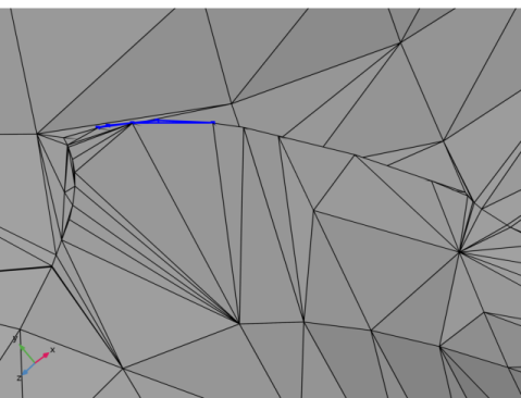
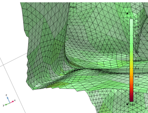
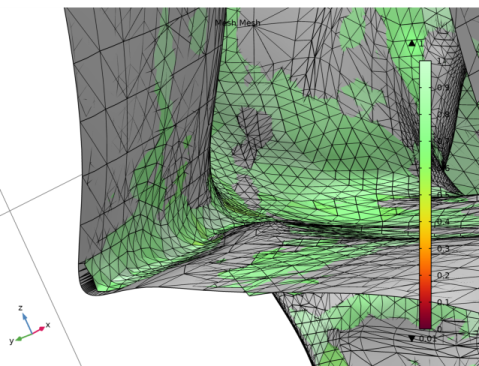
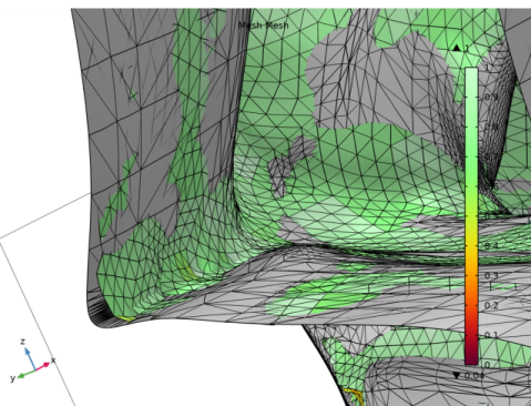
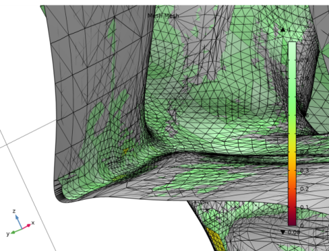
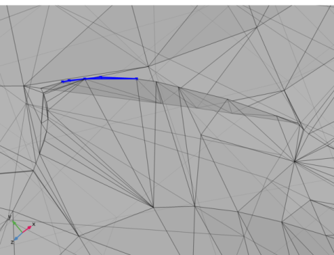
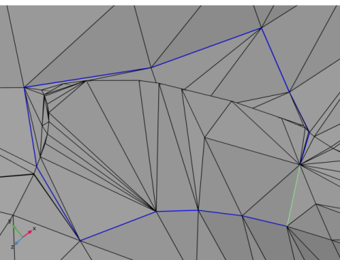
Select mesh edges around the fold by clicking them in the Graphics, similar to what is shown in the image below. The selection is most easily done with tansparancy off. If there are mesh edges on the opposite side of the view or are located inside a closed mesh face, it is recommended to use a Clip Plane or to hide boundaries in the mesh to reach those mesh edges. The selected edges can differ from the ones selected in the figure, as long as the edges form a closed loop, include the fold, and delimit only a small region around the fold. The last requirement is important when generating a new mesh face that follows the original mesh as close as possible.
3
In the Settings window for Create Edges, click  Build Selected to generate the edges and partition the boundary.
Delete Entities 2
1
In the Mesh toolbar, click  Delete Entities.
2
3
In the Settings window for Delete Entities, click  Build Selected.
There is now a hole in the surface mesh, which means that it isn’t possible to create a solid geometry from this mesh. So, before trying to create a geometry again, the hole must be sealed off. Two operations can be used for this purpose: Create Faces and Fill Holes. The Create Faces operation is a manual way of generating mesh faces for holes by selecting edge loops. The Fill Holes operation automatically generates mesh faces to cap several holes at once. In the following tutorial, use the Create Faces operation that generates mesh faces for selected edge loops.
Note that the mesh faces generated by both of these operations will be minimal faces that strive to be as planar as possible.
Create Faces 1
1
In the Mesh toolbar, click  Create Entities and choose Create Faces.
2
3
In the Settings window for Create Faces, click  Build Selected.
The hole is sealed off with a new mesh face that is much smoother.
Join Entities 2
Now, join the two boundaries.
1
In the Mesh toolbar, click  Join Entities.
2
Click in the Graphics window and then press Ctrl+A to select both boundaries.
3
In the Settings window for Join Entities, click  Build Selected.
4
Click the  Go to Default View button in the Graphics toolbar to again see the full mesh.
Mesh Part 1: Length Unit
Before continuing with the geometry, make sure the mesh and geometry have the correct length unit. The meshing sequence in a Mesh Part has a length unit, just as a geometry sequence. Since STL files do not include units, the length unit is set to the default geometry length unit, meter.
1
In the Model Builder window, click Mesh Part 1.
2
In the Settings window for Mesh Part, locate the Units section.
3
Select the Use units check box.
4
From the Length unit list, choose mm.
5
Click  Build All and zoom out to verify that the unit on the axes are indeed set to mm.
Geometry 1
Although the length unit of the Mesh Part 1 sequence now has the correct value, you also need to update the length unit of the Geometry 1 sequence. One way to avoid to update both is to set the length unit of the geometry sequence before importing the file.
1
In the Model Builder window, under Component 1 (comp1) click Geometry 1.
2
In the Settings window for Geometry, locate the Units section.
3
From the Length unit list, choose mm.
Import 1 (imp1)
A rebuild of the Geometry 1 sequence re-imports the geometry from the mesh and updates the length unit.
1
In the Model Builder window, under Component 1 (comp1)>Geometry 1 click Import 1 (imp1).
2
In the Settings window for Import, click  Build Selected.
While waiting for the import to complete, take a look at the Import settings. For large meshes, it can be time consuming to locate and handle irregularities manually. Then, tuning the Simplify mesh parameters can provide an automatic way to simplify the mesh and remove faults to generate smoother geometry faces.
The Relative simplification tolerance is a global tolerance relative to the size of the geometry. If this tolerance is decreased, the generated geometry follows the shape of the original mesh more closely. An increased tolerance will remove larger details and give a more smooth face at the cost of not following the shape of the orignal mesh as closely.
The Defect removal factor is a local tolerance. An increased Defect removal factor removes small irregularities even if they are big relative to the local element size.
At the end of this tutorial, you can find instructions on how to create a mesh plot to see how well the created faces match the source mesh. But first, complete the geometry set up.
The Messages window now reports having imported one solid object, which means that it is time to continue to add a surrounding volume and cut the geometry in half to make use of the symmetry plane. To begin with, modify the orientation of the geometry to improve the visualization.
Rotate 1 (rot1)
1
In the Geometry toolbar, click  Transforms and choose Rotate.
2
Select the object imp1 only, in other words the object for the imported vertebra.
3
In the Settings window for Rotate, locate the Rotation section.
4
From the Axis type list, choose x-axis.
5
In the Angle text field, type 90.
6
Click  Build Selected.
7
Click the  Zoom Extents button in the Graphics toolbar. This will make sure the vertebra is once again in view.
Rotate 2 (rot2)
1
In the Geometry toolbar, click  Transforms and choose Rotate.
2
3
In the Settings window for Rotate, locate the Rotation section.
4
In the Angle text field, type -90.
5
Click  Build Selected.
6
Click the  Zoom Extents button in the Graphics toolbar.
Block 1 (blk1)
In the following section, create a block, combine it with the imported vertebra geometry to create a domain outside of the vertebra, and to cut the geometry in half.
1
In the Geometry toolbar, click  Block.
2
In the Settings window for Block, locate the Size and Shape section.
3
In the Width text field, type 23[mm].
4
In the Depth text field, type 15[mm].
5
In the Height text field, type 15[mm].
6
Locate the Position section. In the x text field, type -22[mm].
7
In the y text field, type -11.1[mm].
8
In the z text field, type 60[mm].
9
Click  Build Selected.
Partition Objects 1 (par1)
1
In the Geometry toolbar, click  Booleans and Partitions and choose Partition Objects.
2
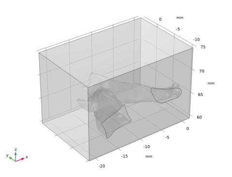
Select the object blk1 only (the block).
3
In the Settings window for Partition Objects, locate the Partition Objects section.
4
Find the Tool objects subsection. Click to select the  Activate Selection toggle button.
5
Select the object rot2 only (the vertebra).
6
Click  Build Selected.
7
Click the  Transparency button in the Graphics toolbar.
8
Click the  Go to Default View button in the Graphics toolbar.
The resulting object now contains two domains, inside and outside the imported geometry. Using a transparent view can help to see the parts inside the block. Continue with finalizing the geometry and creating a mesh.
Form Union (fin)
1
In the Model Builder window, click Form Union (fin).
2
In the Settings window for Form Union/Assembly, click  Build Selected.
Mesh 1
1
In the Model Builder window, under Component 1 (comp1) right-click Mesh 1 and choose Build All.
This builds a tetrahedral mesh on the domains. If this mesh is good enough for the application at hand, it is possible to start setting up the physics at this point. However, many geometries created from mesh require more fine-tuned mesh settings. For example, a specific mesh size setting may cause problems due to the representation of the created face. Then, it often helps to premesh the face with a triangular mesh, restricting the size of the triangles to a more narrow interval. This results in triangles of more similar size and more control over the generated surface mesh. Follow the steps below to generate such a mesh by editing the physics-induced mesh.
2
In the Settings window for Mesh, locate the Sequence Type section.
3
From the list, choose User-controlled mesh.
Size
1
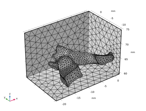
In the Model Builder window, under Component 1 (comp1)>Mesh 1 right-click Size and choose Build Selected.
Building a feature node in the sequence of operations will make sure that any further operation that is added will be placed directly after the built one.
Free Triangular 1
1
In the Mesh toolbar, click  Boundary and choose Free Triangular.
2
Size 1
1
Right-click Free Triangular 1 and choose Size.
2
In the Settings window for Size, locate the Element Size section.
3
Click the Custom button.
4
Locate the Element Size Parameters section. Select the Maximum element size check box.
5
6
Select the Minimum element size check box.
7
This will lower the maximum element size the triangles are allowed to take down to 0.7 mm. In the same way, it will increase the minimum element size allowed to 0.5 mm. The rest of the settings are still taken from the settings of the first Size node in the sequence.
Free Tetrahedral 1
1
In the Model Builder window, under Component 1 (comp1)>Mesh 1 right-click Free Tetrahedral 1 and choose Build All to once again build the mesh on the domains.
Hide some boundaries and turn off transparency to better see the mesh on the boundaries of the vertebra.
2
Click the  Transparency button in the Graphics toolbar.
3
In the Settings window for Free Tetrahedral, locate the Domain Selection section.
4
Click to clear the  Activate Selection toggle button.
5
In the Graphics window toolbar, clicknext to  Select Domains, then choose Select Boundaries.
6
Click the  Click and Hide button in the Graphics toolbar.
7
In the Graphics, click to hide Boundaries 1, 2, and 4, to get the view in the image below.
The mesh is now ready for simulation.
Comparing the Meshed Geometry with the STL Mesh
In order to see how close the meshed geometry follows the source STL mesh, create a plot with both meshes. In this final part of the tutorial you will do this in a new component in the model, and also test the effect of the Simplification tolerance when generating the geometry.
Mesh Part 1
1
In the Model Builder window, under Global Definitions>Mesh Parts click Mesh Part 1.
2
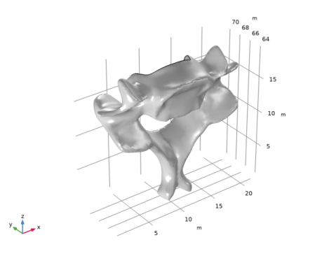
Right-click Global Definitions>Mesh Parts>Mesh Part 1 and choose Create Geometry to reimport the vertebra into a new Component.
Mesh 2
Next, generate a triangular mesh for the vertebra. As the purpose of this part of the tutorial is to check the shape of the face generated by the import, there is no need for a tetrahedral mesh.
Free Triangular 1
1
In the Mesh toolbar, click  Boundary and choose Free Triangular.
2
3
In the Settings window for Free Triangular, click  Build Selected.
Refine 1
Add a Refine operation to further refine the mesh and make sure any curvature is resolved.
1
In the Mesh toolbar, click  Modify and choose Refine.
2
In the Settings window for Refine, locate the Refine Options section.
3
From the Refinement method list, choose Regular refinement.
4
From the Number of refinements list, choose 2.
5
Click  Build Selected.
6
In the Mesh toolbar, click  Plot to automatically create a Mesh dataset and add a Mesh Plot under Results.
Results
Mesh 2
Use the Element Filter option for the Mesh Plot to plot only half of the mesh. This will make it easier to compare the two meshes.
1
In the Settings window for Mesh, click to expand the Element Filter section.
2
Select the Enable filter check box.
3
In the Expression text field, type x>11[mm].
This means that only mesh elements that are located at x coordinates larger than 11 mm will be included in the plot.
4
In the Mesh Plot 1 toolbar, click  Plot.
The generated geometry face is smooth and has a Geometric Shape Order corresponding to the discretization of the physics in the model. In practice, this means that the Geometric Shape Order is most often quadratic, unless solving a CFD problem, where linear discretization is used. To plot the curved elements on the boundary, change the corresponding setting on the dataset.
Mesh 2
1
In the Model Builder window, expand the Results>Datasets node, then click Mesh 2.
2
In the Settings window for Mesh, locate the Mesh section.
3
From the Geometry shape function list, choose Quadratic Lagrange.
To be able to also plot the source STL mesh in the same plot, duplicate the dataset and change the source of the duplicate to the mesh part.
Mesh 3
1
In the Model Builder window, right-click Mesh 2 and choose Duplicate.
2
In the Settings window for Mesh, locate the Mesh section.
3
From the Mesh list, choose Mesh Part 1.
The STL format only supports linear elements, however once imported, a curved representation of the faces is set up if higher order discretization is used in the physics. Therefore, keep the setting Geometry Shape Order: Quadratic Lagrange.
Now that the STL mesh has a dataset, duplicate the Mesh 2 plot feature and modify the settings to point to the newly created dataset.
Mesh 3
1
In the Model Builder window, under Results>Mesh Plot 1 right-click Mesh 2 and choose Duplicate.
2
In the Settings window for Mesh, locate the Data section.
3
From the Dataset list, choose Mesh 3.
4
Locate the Coloring and Style section. From the Element color list, choose Gray.
By giving the source STL mesh a gray color, it will be easier to distinguish between the two meshes. The previously plotted mesh uses the default coloring showing the triangles’ quality with a scale from red (indicating poor quality) to green (good quality).
5
In the Mesh Plot 1 toolbar, click  Plot.
Rotate and zoom in on one of the almost 90 degree corners in the mesh, located in the bottom-left corner of the image below.
It is clear that the mesh of the generated geometry (green) does not follow the source mesh (gray) closely in the region of the 90 degree corner. In regions with lesser curvature the green and gray mesh elements are more intermixed. This indicates better conformance of the generated mesh to the source mesh in those regions.
Now, go back to the Import node and increase the Relative simplification tolerance, to see the effect this has on the generated geometry.
Geometry 2
Import 1 (imp1)
1
In the Model Builder window, under Component 2 (comp2)>Geometry 2 click Import 1 (imp1).
2
In the Settings window for Import, locate the Import section.
3
In the Relative simplification tolerance text field, type 0.02.
4
Click  Build All Objects.
Mesh 2
Free Triangular 1
1
In the Model Builder window, under Component 2 (comp2)>Mesh 2 click Free Triangular 1.
2
In the Settings window for Free Triangular, click  Build All.
Results
Mesh 3
Click somewhere in the Mesh Plot 1 to automatically update the plot.
Looking at the same corner region, the mesh of the generated geometry (green) shows a more rough representation of the source mesh (grey). This is expected as increasing the Relative simplification factor allows for a larger deviation from the source mesh when the surfaces of the geometry are generated during the import.
This time, go back and decrease the Relative simplification tolerance to 0.001. This is 10 times smaller than the default value of 0.01.
Geometry 2
Import 1 (imp1)
1
In the Model Builder window, under Component 2 (comp2)>Geometry 2 click Import 1 (imp1).
2
In the Settings window for Import, locate the Import section.
3
In the Relative simplification tolerance text field, type 0.001.
4
Click  Build All Objects.
Mesh 2
Free Triangular 1
1
In the Model Builder window, under Component 2 (comp2)>Mesh 2 click Free Triangular 1.
2
In the Settings window for Free Triangular, click  Build All.
Results
Mesh 3
Click somewhere in the Mesh Plot 1 to automatically update the plot.
The mesh of the generated geometry (green) now follows the source mesh (gray) much closer. This is the effect of the smaller Relative simplification factor, which allows for less deviation from the source mesh when the surface is generated during import.
 

1
The STL geometry is provided courtesy of Mark Yeoman, Continuum Blue, UK.