PDF

Submodeling Analysis of a Shaft
Introduction
Submodeling can be used when it is not possible to resolve all details of a complex geometry in a global model.
You can cope with this type of problems with a technique known as submodeling. First you solve the complete model with a mesh which is sufficient to capture the stiffness of the structure. In a second analysis you create a local model (submodel) of the region around the stress concentration with a fine mesh, and solve it using the displacements from the global model as boundary conditions.
There are some underlying assumptions when using submodels:
In this example this technique is applied to perform an accurate stress evaluation in a structural mechanics model, but the same approach is applicable to many physical problems. The example geometry as such is not so complicated, so there is nothing to gain from a submodeling in this case. The purpose of the example is to show the technique.
Model Definition
The geometry consists of a shaft with a sudden change in diameter. At the location of the diameter change, there is a fillet with a small radius. In the fillet, stress concentrations will appear. There is also a central hole through the shaft. The geometry and mesh are shown in Figure 1.
The shaft is fixed at the thick end. On the thin end, a tensile force of 300 N and a shear force of 100 N are applied.
Figure 1: The full model.
As submodel, a region around the fillet at side giving the highest stress is chosen. The cuts where the boundary conditions are applied on the submodel should preferably be placed at locations where the stress field is fairly smooth.
The geometry and mesh of the submodel are shown in Figure 2. As can be seen, the fillet has a very good mesh resolution since the purpose is to obtain results with high accuracy there.
Figure 2: The submodel.
Results
The general stress distribution is shown in Figure 3. Since the load is unsymmetrical (there is both an axial and a bending component), the highest stress occurs at the side with positive Z coordinate.
The cut through the model in Figure 4 displays that the stresses are not well resolved. There are significant jumps between the neighboring elements.
In the corresponding figures from the submodel, Figure 5 and Figure 6, the stress field is smooth and well resolved.
The computed peak stress for the global model is about 9% different compared to that in the submodel, which is expected given the coarse mesh in the global model.
Figure 3: Stress distribution in the global model.
Figure 4: Stress within the full model (cut view).
Figure 5: Stress distribution in the submodel.
Figure 6: Stress within the submodel (cut view).
As a verification, it is a good habit to always check the stress state at the cuts where the submodel has displacements prescribed by the results in the global model. Such a comparison is shown in Figure 7. The results have an almost perfect match, which strongly indicates that the submodel has been set up correctly.
Figure 7: Stress distribution over one of the cuts. Global model (left) and submodel (right) are compared.
Notes About the COMSOL Implementation
Two different components are used within the same mph file. In the global model, a general extrusion feature is introduced in order to describe the mapping of results from the global model to the submodel. The prescribed displacements on the cut boundaries in the submodel reference the displacements in the global model through this mapping.
In this example, there are no volume forces. If there were, such forces must be applied also on the submodel.
Application Library path: COMSOL_Multiphysics/Structural_Mechanics/shaft_submodeling
Modeling Instructions
From the File menu, choose New.
New
In the New window, click  Model Wizard.
Model Wizard
1
In the Model Wizard window, click  3D.
2
In the Select Physics tree, select Structural Mechanics>Solid Mechanics (solid).
3
Click Add.
4
Click  Study.
5
In the Select Study tree, select General Studies>Stationary.
6
Geometry 1
In the Model Builder window, under Component 1 (comp1) right-click Geometry 1 and choose 3D Part.
Full Geometry
Create the geometry. To simplify this step, insert a prepared geometry sequence.
1
In the Settings window for Part, locate the Units section.
2
From the Length unit list, choose mm.
3
In the Geometry toolbar, click Insert Sequence and choose Insert Sequence.
4
5
In the Geometry toolbar, click  Build All.
6
In the Label text field, type Full Geometry.
Full model
1
In the Model Builder window, click Component 1 (comp1).
2
In the Settings window for Component, type Full model in the Label text field.
Geometry 1
1
In the Model Builder window, under Full model (comp1) click Geometry 1.
2
In the Settings window for Geometry, locate the Units section.
3
From the Length unit list, choose mm.
Full Geometry 1 (pi1)
1
In the Geometry toolbar, click  Parts and choose Full Geometry.
2
In the Settings window for Part Instance, click  Build All Objects.
3
Click to expand the Boundary Selections section. In the table, enter the following settings:
The geometry sequence contains two selections, these will be used later to apply loads and constraints.
Add Material
1
In the Home toolbar, click  Add Material to open the Add Material window.
2
Go to the Add Material window.
3
In the tree, select Built-in>Structural steel.
4
Right-click and choose Add to Global Materials.
5
In the Home toolbar, click  Add Material to close the Add Material window.
The material is now defined as global material so that both the full model and the submodel can use the same material definition, defined at one location only in the model tree.
Materials
Material Link 1 (matlnk1)
In the Model Builder window, under Full model (comp1) right-click Materials and choose More Materials>Material Link.
Solid Mechanics (solid)
Fixed Constraint 1
1
In the Model Builder window, under Full model (comp1) right-click Solid Mechanics (solid) and choose Fixed Constraint.
2
In the Settings window for Fixed Constraint, locate the Boundary Selection section.
3
From the Selection list, choose Fixed Constrained (Full Geometry 1).
Boundary Load 1
1
In the Physics toolbar, click  Boundaries and choose Boundary Load.
2
In the Settings window for Boundary Load, locate the Boundary Selection section.
3
From the Selection list, choose Boundary Load (Full Geometry 1).
4
Locate the Force section. From the Load type list, choose Total force.
5
Specify the Ftot vector as
Mesh 1
1
In the Model Builder window, under Full model (comp1) click Mesh 1.
2
In the Settings window for Mesh, locate the Physics-Controlled Mesh section.
3
From the Element size list, choose Coarse.
4
Click  Build All.
5
Click the  Zoom Extents button in the Graphics toolbar.
Full model
1
In the Model Builder window, click Study 1.
2
In the Settings window for Study, type Full model in the Label text field.
3
In the Home toolbar, click  Compute.
Results
Stress - Full model
1
In the Settings window for 3D Plot Group, type Stress - Full model in the Label text field.
2
Locate the Color Legend section. Select the Show maximum and minimum values check box.
Volume 1
1
In the Model Builder window, expand the Stress - Full model node, then click Volume 1.
2
In the Settings window for Volume, click to expand the Quality section.
3
From the Resolution list, choose No refinement.
4
From the Smoothing list, choose None.
5
In the Stress - Full model toolbar, click  Plot.
6
Click the  Zoom Extents button in the Graphics toolbar.
Cut Plane 1
1
In the Model Builder window, expand the Results>Datasets node.
2
Right-click Results>Datasets and choose Cut Plane.
3
In the Settings window for Cut Plane, locate the Plane Data section.
4
From the Plane list, choose XZ-planes.
Cut Plane Stress -Full model
1
In the Results toolbar, click  2D Plot Group.
2
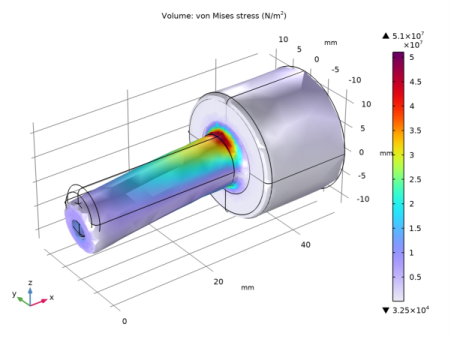
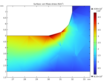
In the Settings window for 2D Plot Group, type Cut Plane Stress -Full model in the Label text field.
3
Locate the Color Legend section. Select the Show maximum and minimum values check box.
Surface 1
1
Right-click Cut Plane Stress -Full model and choose Surface.
2
In the Settings window for Surface, locate the Expression section.
3
In the Expression text field, type solid.mises.
4
Click to expand the Quality section. From the Resolution list, choose No refinement.
5
From the Smoothing list, choose None.
6
In the Cut Plane Stress -Full model toolbar, click  Plot.
7
In the Model Builder window, expand the Results>Views node.
Axis
1
In the Model Builder window, expand the Results>Views>View 2D 4 node, then click Axis.
2
In the Settings window for Axis, locate the Axis section.
3
In the x minimum text field, type 25.8.
4
In the x maximum text field, type 34.2.
5
In the y minimum text field, type 1.5.
6
In the y maximum text field, type 7.5.
7
Click  Update.
Add Component
In the Model Builder window, right-click the root node and choose Add Component>3D.
Submodel
In the Settings window for Component, type Submodel in the Label text field.
Submodel Cut
1
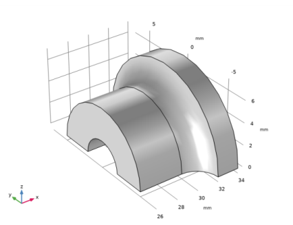
In the Model Builder window, under Global Definitions right-click Geometry Parts and choose 3D Part.
2
In the Settings window for Part, type Submodel Cut in the Label text field.
3
Locate the Units section. From the Length unit list, choose mm.
Cylinder 1 (cyl1)
1
In the Geometry toolbar, click  Cylinder.
2
In the Settings window for Cylinder, locate the Size and Shape section.
3
In the Radius text field, type 7.
4
In the Height text field, type 8.
5
Locate the Position section. In the x text field, type 26.
6
Locate the Axis section. From the Axis type list, choose x-axis.
Block 1 (blk1)
1
In the Geometry toolbar, click  Block.
2
In the Settings window for Block, locate the Size and Shape section.
3
In the Width text field, type 10.
4
In the Depth text field, type 14.
5
In the Height text field, type 10.
6
Locate the Position section. In the x text field, type 26.
7
In the y text field, type -7.
Submodel Cut
1
In the Geometry toolbar, click  Booleans and Partitions and choose Intersection.
2
In the Settings window for Intersection, type Submodel Cut in the Label text field.
3
Click in the Graphics window and then press Ctrl+A to select both objects.
4
Locate the Selections of Resulting Entities section. Select the Resulting objects selection check box.
5
From the Show in instances list, choose Boundary selection.
Geometry 2
1
In the Model Builder window, under Submodel (comp2) click Geometry 2.
2
In the Settings window for Geometry, locate the Units section.
3
From the Length unit list, choose mm.
Full Geometry 1 (pi1)
In the Geometry toolbar, click  Parts and choose Full Geometry.
Submodel Cut 1 (pi2)
1
In the Geometry toolbar, click  Parts and choose Submodel Cut.
2
In the Settings window for Part Instance, click  Build Selected.
3
Locate the Boundary Selections section. In the table, enter the following settings:
Intersection 1 (int1)
1
In the Geometry toolbar, click  Booleans and Partitions and choose Intersection.
2
Click in the Graphics window and then press Ctrl+A to select both objects.
3
In the Settings window for Intersection, click  Build All Objects.
The submodel geometry is now built. In order to create a structured mesh, you need to partition the geometry following the xz-plane.
Work Plane 1 (wp1)
1
In the Geometry toolbar, click  Work Plane.
2
In the Settings window for Work Plane, locate the Plane Definition section.
3
From the Plane list, choose zx-plane.
Partition Objects 1 (par1)
1
In the Geometry toolbar, click  Booleans and Partitions and choose Partition Objects.
2
3
In the Settings window for Partition Objects, locate the Partition Objects section.
4
From the Partition with list, choose Work plane.
Mesh Control Domains 1 (mcd1)
1
In the Geometry toolbar, click  Virtual Operations and choose Mesh Control Domains.
2
On the object fin, select Domains 1 and 2 only.
3
In the Geometry toolbar, click  Build All.
4
Click the  Zoom Extents button in the Graphics toolbar.
Materials
Material Link 2 (matlnk2)
In the Model Builder window, under Submodel (comp2) right-click Materials and choose More Materials>Material Link.
Add Physics
1
In the Home toolbar, click  Add Physics to open the Add Physics window.
2
Go to the Add Physics window.
3
In the tree, select Structural Mechanics>Solid Mechanics (solid).
4
Find the Physics interfaces in study subsection. In the table, select the Solve check box for Full model.
5
Click Add to Submodel in the window toolbar.
6
In the Home toolbar, click  Add Physics to close the Add Physics window.
Definitions (comp1)
In the Model Builder window, under Full model (comp1) click Definitions.
General Extrusion 1 (genext1)
1
In the Definitions toolbar, click  Nonlocal Couplings and choose General Extrusion.
2
3
In the Settings window for General Extrusion, locate the Destination Map section.
4
In the x-expression text field, type X.
5
In the y-expression text field, type Y.
6
In the z-expression text field, type Z.
7
Locate the Source section. From the Source frame list, choose Material  (X, Y, Z).
You have now created the nonlocal coupling which will be used for mapping the solution from the full model to the submodel.
Solid Mechanics 2 (solid2)
In the Model Builder window, under Submodel (comp2) click Solid Mechanics 2 (solid2).
Prescribed Displacement 1
1
In the Physics toolbar, click  Boundaries and choose Prescribed Displacement.
2
In the Settings window for Prescribed Displacement, locate the Boundary Selection section.
3
From the Selection list, choose Submodel Cut (Submodel Cut 1).
4
Locate the Prescribed Displacement section. Select the Prescribed in x direction check box.
5
In the u0x text field, type comp1.genext1(comp1.u).
6
Select the Prescribed in y direction check box.
7
In the u0y text field, type comp1.genext1(comp1.v).
8
Select the Prescribed in z direction check box.
9
In the u0z text field, type comp1.genext1(comp1.w).
Mesh 2
Mapped 1
1
In the Mesh toolbar, click  Boundary and choose Mapped.
2
Distribution 1
1
Right-click Mapped 1 and choose Distribution.
2
3
In the Settings window for Distribution, locate the Distribution section.
4
From the Distribution type list, choose Predefined.
5
In the Number of elements text field, type 6.
6
In the Element ratio text field, type 3.
7
Select the Reverse direction check box.
Distribution 2
1
In the Model Builder window, right-click Mapped 1 and choose Distribution.
2
3
In the Settings window for Distribution, locate the Distribution section.
4
From the Distribution type list, choose Predefined.
5
In the Number of elements text field, type 6.
6
In the Element ratio text field, type 3.
Distribution 3
1
Right-click Mapped 1 and choose Distribution.
2
3
In the Settings window for Distribution, locate the Distribution section.
4
In the Number of elements text field, type 6.
Distribution 4
1
Right-click Mapped 1 and choose Distribution.
2
3
In the Settings window for Distribution, locate the Distribution section.
4
From the Distribution type list, choose Predefined.
5
In the Number of elements text field, type 10.
6
In the Element ratio text field, type 2.
Swept 1
In the Mesh toolbar, click  Swept.
Distribution 1
1
Right-click Swept 1 and choose Distribution.
2
In the Settings window for Distribution, locate the Distribution section.
3
In the Number of elements text field, type 12.
4
Click  Build All.
5
In the Model Builder window, right-click Mesh 2 and choose Build All.
6
Click the  Zoom Extents button in the Graphics toolbar.
Add Study
1
In the Home toolbar, click  Add Study to open the Add Study window.
2
Go to the Add Study window.
3
Find the Studies subsection. In the Select Study tree, select General Studies>Stationary.
4
Find the Physics interfaces in study subsection. In the table, clear the Solve check box for Solid Mechanics (solid).
5
Click Add Study in the window toolbar.
6
In the Model Builder window, click the root node.
7
In the Home toolbar, click  Add Study to close the Add Study window.
Submodel
In the Settings window for Study, type Submodel in the Label text field.
Step 1: Stationary
1
In the Model Builder window, under Submodel click Step 1: Stationary.
2
In the Settings window for Stationary, click to expand the Values of Dependent Variables section.
3
Find the Values of variables not solved for subsection. From the Settings list, choose User controlled.
4
From the Method list, choose Solution.
5
From the Study list, choose Full model, Stationary.
6
In the Home toolbar, click  Compute.
Results
Stress - Submodel
1
In the Settings window for 3D Plot Group, type Stress - Submodel in the Label text field.
2
Locate the Color Legend section. Select the Show maximum and minimum values check box.
Volume 1
1
In the Model Builder window, expand the Stress - Submodel node, then click Volume 1.
2
In the Settings window for Volume, locate the Quality section.
3
From the Resolution list, choose No refinement.
4
From the Smoothing list, choose None.
5
In the Stress - Submodel toolbar, click  Plot.
6
Click the  Zoom Extents button in the Graphics toolbar.
Cut Plane 2
1
In the Results toolbar, click  Cut Plane.
2
In the Settings window for Cut Plane, locate the Plane Data section.
3
From the Plane list, choose XZ-planes.
4
Locate the Data section. From the Dataset list, choose Submodel/Solution 2 (3) (sol2).
Cut Plane Stress - Submodel
1
In the Results toolbar, click  2D Plot Group.
2
In the Settings window for 2D Plot Group, type Cut Plane Stress - Submodel in the Label text field.
3
Locate the Color Legend section. Select the Show maximum and minimum values check box.
4
Locate the Data section. From the Dataset list, choose Cut Plane 2.
Surface 1
1
Right-click Cut Plane Stress - Submodel and choose Surface.
2
In the Settings window for Surface, locate the Expression section.
3
In the Expression text field, type solid2.mises.
4
Locate the Quality section. From the Resolution list, choose No refinement.
5
From the Smoothing list, choose None.
6
In the Cut Plane Stress - Submodel toolbar, click  Plot.
7
Click the  Zoom Extents button in the Graphics toolbar.
Now verify that the differences in stress between the full model and the submodel are small where the displacements are mapped.
Cut Plane 3
1
In the Results toolbar, click  Cut Plane.
2
In the Settings window for Cut Plane, locate the Plane Data section.
3
In the X-coordinate text field, type 26.
Stress comparison
1
In the Results toolbar, click  2D Plot Group.
2
In the Settings window for 2D Plot Group, type Stress comparison in the Label text field.
3
Locate the Data section. From the Dataset list, choose None.
Surface 1
1
Right-click Stress comparison and choose Surface.
2
In the Settings window for Surface, locate the Data section.
3
From the Dataset list, choose Cut Plane 3.
4
Locate the Expression section. In the Expression text field, type solid.mises.
5
Locate the Quality section. From the Resolution list, choose No refinement.
6
From the Smoothing list, choose None.
7
In the Stress comparison toolbar, click  Plot.
8
In the Results toolbar, click  More Datasets and choose Surface.
Surface 1
1
In the Settings window for Surface, locate the Data section.
2
From the Dataset list, choose Submodel/Solution 2 (3) (sol2).
3
4
Locate the Parameterization section. From the x- and y-axes list, choose YZ-plane.
Surface 2
1
In the Model Builder window, right-click Stress comparison and choose Surface.
2
In the Settings window for Surface, locate the Data section.
3
From the Dataset list, choose Surface 1.
4
Locate the Expression section. In the Expression text field, type solid2.mises.
5
Locate the Quality section. From the Resolution list, choose No refinement.
6
From the Smoothing list, choose None.
7
Click to expand the Inherit Style section. From the Plot list, choose Surface 1.
Deformation 1
1
Right-click Surface 2 and choose Deformation.
2
In the Settings window for Deformation, locate the Expression section.
3
In the x component text field, type 11.
4
In the y component text field, type 0.
5
Locate the Scale section. Select the Scale factor check box.
6
7
In the Stress comparison toolbar, click  Plot.
8
Click the  Zoom Extents button in the Graphics toolbar.
The solution is computed, follow the steps below if you want to save and reuse the model in the future.
Full model
Step 1: Stationary
1
In the Model Builder window, under Full model click Step 1: Stationary.
2
In the Settings window for Stationary, locate the Physics and Variables Selection section.
3
In the table, clear the Solve for check box for Solid Mechanics 2 (solid2).