|
|
|

|
1
|
|
2
|
In the Select Physics tree, select Acoustics>Pressure Acoustics>Pressure Acoustics, Frequency Domain (acpr).
|
|
3
|
Click Add.
|
|
4
|
Click
|
|
5
|
|
6
|
Click
|
|
1
|
|
2
|
|
3
|
Click Browse.
|
|
4
|
Browse to the model’s Application Libraries folder and double-click the file eigenmodes_of_room.mphbin.
|
|
5
|
Click Import.
|
|
6
|
|
1
|
In the Model Builder window, under Component 1 (comp1) right-click Materials and choose Blank Material.
|
|
2
|
|
4
|
|
1
|
|
2
|
|
3
|
|
4
|
|
1
|
|
2
|
|
3
|
|
4
|
|
1
|
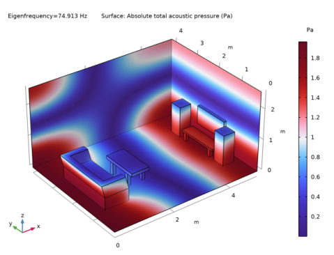
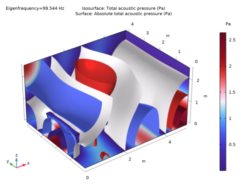
In the Model Builder window, expand the Results>Acoustic Pressure (acpr) node, then click Surface 1.
|
|
2
|
In the Settings window for Surface, click Replace Expression in the upper-right corner of the Expression section. From the menu, choose Component 1 (comp1)>Pressure Acoustics, Frequency Domain>Pressure and sound pressure level>acpr.absp_t - Absolute total acoustic pressure - Pa.
|
|
3
|
|
4
|
|
5
|
|
1
|
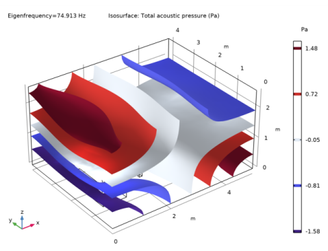
In the Model Builder window, expand the Acoustic Pressure, Isosurfaces (acpr) node, then click Isosurface 1.
|
|
2
|
|
3
|
|
4
|
|
1
|
|
2
|
|
3
|
|
1
|
|
2
|
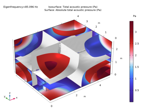
In the Settings window for Surface, click Replace Expression in the upper-right corner of the Expression section. From the menu, choose Component 1 (comp1)>Pressure Acoustics, Frequency Domain>Pressure and sound pressure level>acpr.absp_t - Absolute total acoustic pressure - Pa.
|
|
3
|
|
4
|
|
1
|
|
2
|
|
3
|
|
1
|
|
2
|
|
3
|
|
4
|