PDF

Slip Flow Benchmark
Introduction
As the absolute pressure in a gas flow is reduced, the mean free path of the gas molecules begins to approach the size of the vessel through which the flow occurs. Such rarefied flows are characterized by a parameter known as the Knudsen number, which is the ratio of the mean free path to the characteristic length of the geometry. In a rarefied flow the gas cannot be treated as a continuum and the kinetic nature of the flow must be considered. However, at moderate Knudsen numbers between approximately 0.01 and 0.1, the flow can be modeled using the Navier-Stokes equations, except in a thin region adjacent to the walls, termed the Knudsen layer. This regime is termed the slip flow regime. In the slip flow regime the Knudsen layer can be replaced by alternative boundary conditions for the Navier-Stokes equations. A slip velocity along the geometry walls develops, and the temperature at the walls of the structure becomes discontinuous at this level of approximation. Phenomena such as viscous slip and thermal creep or transpiration become important.
This model is a benchmark model for COMSOL’s Slip Flow interface. It is based on analytic and numeric calculations presented in Ref. 1. Air at atmospheric pressure flows through a conducting microchannel connecting two reservoirs maintained at different temperatures. A flow between the two reservoirs develops as a result of thermal creep along the channel wall, which in turn produces a pressure gradient. At steady state the net flow through the channel is zero, but a pressure gradient exists between the hot and cold sides of the reservoir and a circulating flow occurs.
Model Definition
The model consists of two chambers 7.5 μm by 15 μm, with a depth significantly larger than either of these dimensions (this means that the simulation can be performed using the 2D XY interface). The chambers are linked by a narrow channel of the same depth with width 1.5 μm and length 15 μm. The chamber and channel walls are fabricated from silicon and have a thickness of 1 μm. The walls of the two chambers are in thermal contact with heat sinks maintained at 300 K and 400 K, respectively. The channel walls are thermally insulated. Figure 1 shows the model geometry. The gas in the center of the channel is at a pressure of 1 atmosphere.
Figure 1: The Model Geometry
For channels of micron scale dimensions the Knudsen number becomes greater than 0.01 even at atmospheric pressure. It is therefore necessary to use a slip condition on the surfaces of walls in the vicinity of the channel.
Slip Wall Boundary Condition
The slip velocity, uslip, along the walls of the channel is given by (Ref. 2):
(1)
where λ is the mean free path of the gas, n is the boundary normal, τ is the viscous stress tensor, Tw is the wall temperature, Tg is the temperature of the gas, μ is its viscosity, and ρ is its density. The slip coefficients: σs (the viscous slip coefficient), σT (the thermal slip coefficient), and ζT (the temperature jump coefficient) can be defined by material properties and the tangential momentum accommodation coefficient, av, within a generalized form of Maxwell’s original slip model (see Ref. 2 and Ref. 3). For a model in which the surface reflects some molecules diffusely and some specularly, av is the fraction of molecules which are reflected diffusely. Within Maxwell’s model the slip coefficients are:
where κ is the thermal conductivity of the gas.
The mean free path can be computed from the gas properties using the following equation (Ref. 2):
Results and Discussion
Figure 2 shows the mean free path of the gas throughout the simulation domain. Since the channel width is 1.5 μm, a mean free path of 75 nm corresponds to a Knudsen number of 0.05. This value is comparable to the Knudsen number of the gas in the channel and is within the slip flow regime.
The velocity of the gas in the x-direction is shown in Figure 3, together with the velocity streamlines. In the steady state there is no net flow through the channel, but a flow parallel to the walls, in the direction of the thermal gradient (cold to hot), develops due to thermal creep. To compensate for this flow a back flow develops in the center of the channel, which is driven by a pressure gradient in the gas.
The temperature distribution in the channels is shown in Figure 4. The thermal gradient is predominately parallel to the walls, however there are some normal thermal gradients in the vicinity of the opening to the channel, which result in a temperature jump between the gas and the wall, according to Equation 1. This temperature jump simulates the effect of the Knudsen layer, which is not captured by the continuum Navier-Stokes equations.
Figure 2: Gas mean free path. The channel width is 1.5 μm, so the Knudsen number varies between 0.064 and 0.045.
Figure 3: x-velocity (color) and streamlines (white) inside the channel. Flow is driven by thermal creep along the walls of the channel but a back-flow, driven by the pressure difference between the reservoirs, occurs in the center of the channel.
Figure 4: Temperature contours within the model. Note that a temperature jump occurs between the vessel walls and the gas when normal heat fluxes occur into the wall from the gas.
Figure 5: Pressure on the wall of the channel, as a function of position.
Figure 5 shows the relative pressure acting on the channel wall, as a function of position along the wall. The pressure is lowest in the coolest chamber, at 151 Pa below atmospheric, and highest in the warmer chamber, at 179 Pa above atmospheric pressure. The asymmetry of the pressure distribution about the center of the channel results from changes in the number density of the gas in the two reservoirs. The total pressure difference of 330 Pa is similar to the value predicted in Ref. 1 for a numerical simulation of an equivalent problem (336 Pa), and is also in good agreement with the value predicted by the analytic model of Ref. 1, which is (335 Pa). This model therefore serves as a benchmark for the Slip Flow interface.
References
1. G. Kariadakis, A. Beskok, and N. Aluru, Microflows and Nanoflows, Springer Science and Business Media, 2005.
2. E.H. Kennard, Kinetic Theory of Gases, McGraw-Hill, New York, 1938.
3. J.C. Maxwell, “On Stresses in Rarefied Gases Arising from Inequalities of Temperature”, Phil. Trans. R. Soc. Lond., vol. 170, pp. 231–256, 1879.
Application Library path: Microfluidics_Module/Rarefied_Flow/slip_flow_benchmark
Modeling Instructions
From the File menu, choose New.
New
In the New window, click  Model Wizard.
Model Wizard
1
In the Model Wizard window, click  2D.
2
In the Select Physics tree, select Fluid Flow>Rarefied Flow>Slip Flow (slpf).
3
Click Add.
4
Click  Study.
5
In the Select Study tree, select General Studies>Stationary.
6
Geometry 1
Change the length units to μm and specify the geometry.
1
In the Model Builder window, under Component 1 (comp1) click Geometry 1.
2
In the Settings window for Geometry, locate the Units section.
3
From the Length unit list, choose µm.
Rectangle 1 (r1)
1
In the Geometry toolbar, click  Rectangle.
2
In the Settings window for Rectangle, locate the Size and Shape section.
3
In the Width text field, type 15.
4
In the Height text field, type 1.5.
5
Locate the Position section. In the y text field, type -0.75.
Rectangle 2 (r2)
1
In the Geometry toolbar, click  Rectangle.
2
In the Settings window for Rectangle, locate the Size and Shape section.
3
In the Width text field, type 7.5.
4
In the Height text field, type 15.
5
Locate the Position section. In the x text field, type -7.5.
6
In the y text field, type -7.5.
Rectangle 3 (r3)
1
In the Geometry toolbar, click  Rectangle.
2
In the Settings window for Rectangle, locate the Size and Shape section.
3
In the Width text field, type 7.5.
4
In the Height text field, type 15.
5
Locate the Position section. In the x text field, type 15.
6
In the y text field, type -7.5.
Union 1 (uni1)
1
In the Geometry toolbar, click  Booleans and Partitions and choose Union.
2
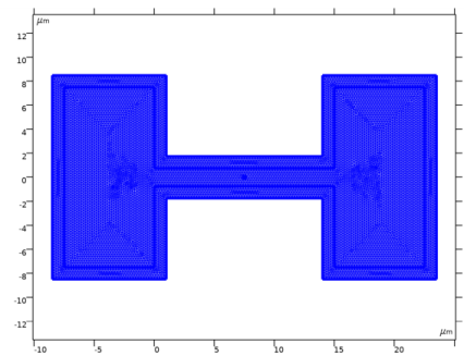
Click in the Graphics window and then press Ctrl+A to select all objects.
3
In the Settings window for Union, locate the Union section.
4
Clear the Keep interior boundaries check box.
5
Click the  Zoom Extents button in the Graphics toolbar.
Rectangle 4 (r4)
1
In the Geometry toolbar, click  Rectangle.
2
In the Settings window for Rectangle, locate the Size and Shape section.
3
In the Width text field, type 9.5.
4
In the Height text field, type 17.
5
Locate the Position section. In the x text field, type -8.5.
6
In the y text field, type -8.5.
Rectangle 5 (r5)
1
In the Geometry toolbar, click  Rectangle.
2
In the Settings window for Rectangle, locate the Size and Shape section.
3
In the Width text field, type 15.
4
In the Height text field, type 3.5.
5
Locate the Position section. In the y text field, type -1.75.
Rectangle 6 (r6)
1
In the Geometry toolbar, click  Rectangle.
2
In the Settings window for Rectangle, locate the Size and Shape section.
3
In the Width text field, type 9.5.
4
In the Height text field, type 17.
5
Locate the Position section. In the x text field, type 14.
6
In the y text field, type -8.5.
Union 2 (uni2)
1
In the Geometry toolbar, click  Booleans and Partitions and choose Union.
2
Select the objects r4, r5, and r6 only.
3
In the Settings window for Union, locate the Union section.
4
Clear the Keep interior boundaries check box.
Point 1 (pt1)
1
In the Geometry toolbar, click  Point.
2
In the Settings window for Point, locate the Point section.
3
In the x text field, type 7.5.
4
Click  Build All Objects.
5
Click the  Zoom Extents button in the Graphics toolbar.
Specify the material properties for the cavity walls and the gas.
Add Material
1
In the Home toolbar, click  Add Material to open the Add Material window.
2
Go to the Add Material window.
3
4
Click Add to Component in the window toolbar.
5
In the tree, select Built-in>Silicon.
6
Click Add to Component in the window toolbar.
7
In the Home toolbar, click  Add Material to close the Add Material window.
Materials
Silicon (mat2)
Select Domain 1 only.
Slip Flow (slpf)
Set the physics for the solid regions to be the heat transfer equation.
Solid 1
1
In the Model Builder window, under Component 1 (comp1) right-click Slip Flow (slpf) and choose the domain setting Heat Transfer>Solid.
2
Apply thermal insulation on the boundaries of the connecting duct.
Thermal Insulation 1
1
In the Physics toolbar, click  Boundaries and choose Thermal Insulation.
2
Fix the temperature on the walls of the two reservoirs.
Temperature 1
1
In the Physics toolbar, click  Boundaries and choose Temperature.
2
3
In the Settings window for Temperature, locate the Temperature section.
4
In the T0 text field, type 300[K].
Temperature 2
1
In the Physics toolbar, click  Boundaries and choose Temperature.
2
3
In the Settings window for Temperature, locate the Temperature section.
4
In the T0 text field, type 400[K].
Apply slip boundary conditions near and inside the channel.
Slip Wall 1
1
In the Physics toolbar, click  Boundaries and choose Slip Wall.
2
In the Settings window for Slip Wall, locate the Boundary Selection section.
3
From the Selection list, choose All boundaries.
Apply a pressure constraint in the center of the channel.
Pressure Point Constraint 1
1
In the Physics toolbar, click  Points and choose Pressure Point Constraint.
2
Set up the mesh.
Mesh 1
Size 1
1
In the Model Builder window, under Component 1 (comp1) right-click Mesh 1 and choose Size.
2
In the Settings window for Size, locate the Element Size section.
3
From the Calibrate for list, choose Fluid dynamics.
4
From the Predefined list, choose Extra fine.
Free Triangular 1
1
In the Mesh toolbar, click  Free Triangular.
2
In the Settings window for Free Triangular, click  Build All.
Study 1
In the Home toolbar, click  Compute.
Results
Velocity (slpf)
Plot the mean free path number in the domain to check the Knudsen number.
Mean Free Path
1
In the Home toolbar, click  Add Plot Group and choose 2D Plot Group.
2
Right-click 2D Plot Group 5 and choose Rename.
3
In the Rename 2D Plot Group dialog box, type Mean Free Path in the New label text field.
4
Surface 1
1
Right-click Mean Free Path and choose Surface.
2
In the Settings window for Surface, locate the Expression section.
3
In the Expression text field, type slpf.lambda.
4
In the Mean Free Path toolbar, click  Plot.
5
Click the  Zoom Extents button in the Graphics toolbar.
Compare the resulting plot with Figure 2.
Plot the x-velocity and streamlines in the domain.
x-Velocity, Streamlines
1
In the Model Builder window, right-click Velocity (slpf) and choose Duplicate.
2
Right-click Velocity (slpf) 1 and choose Rename.
3
In the Rename 2D Plot Group dialog box, type x-Velocity, Streamlines in the New label text field.
4
Streamline 1
1
Right-click x-Velocity, Streamlines and choose Streamline.
2
In the Settings window for Streamline, locate the Streamline Positioning section.
3
From the Positioning list, choose Magnitude controlled.
4
In the Density text field, type 12.
5
Locate the Coloring and Style section. Find the Point style subsection. From the Color list, choose White.
Surface
1
In the Model Builder window, click Surface.
2
In the Settings window for Surface, locate the Expression section.
3
In the Expression text field, type u.
4
In the x-Velocity, Streamlines toolbar, click  Plot.
Compare the resulting plot with Figure 3.
Plot the Temperature in the domain.
Contour
1
In the Model Builder window, expand the Isothermal Contours (slpf) node, then click Contour.
2
In the Settings window for Contour, locate the Levels section.
3
In the Total levels text field, type 40.
4
In the Isothermal Contours (slpf) toolbar, click  Plot.
5
Locate the Coloring and Style section. From the Color table list, choose Rainbow.
Compare the resulting plot with Figure 4.
Plot the pressure along the channel wall.
Channel Pressure
1
In the Home toolbar, click  Add Plot Group and choose 1D Plot Group.
2
Right-click 1D Plot Group 7 and choose Rename.
3
In the Rename 1D Plot Group dialog box, type Channel Pressure in the New label text field.
4
Line Graph 1
1
Right-click Channel Pressure and choose Line Graph.
2
3
In the Settings window for Line Graph, locate the y-Axis Data section.
4
In the Expression text field, type p.
5
In the Channel Pressure toolbar, click  Plot.
Compare the resulting plot with Figure 5.