PDF

Nonisothermal Laminar Flow in a Circular Tube
Introduction
This validation model of laminar airflow through a tube validates the heat transfer coefficient obtained from the simulation against Nusselt-number-based correlation functions. The simulation results are in good agreement with experimental measurements.
Model Definition
The tube is modeled as a 2D axisymmetric geometry. The tube has a diameter of 0.05 m and a length of 3 m. A coupled heat transfer and fluid flow problem is solved using the Nonisothermal Flow interface.
At the inlet, a laminar velocity profile U with an average velocity Uav of 0.1 m/s is applied using the normal inflow option:
where r denotes the radial distance from the tube center and b the tube’s diameter. The expression gives the typical parabolic velocity profile for fully developed laminar flow. The air enters with a temperature T0 of 283 K.
At the cylinder wall, a constant heat flux qw of 10 W/m² is applied.
Nusselt Number Correlations
Two different Nusselt number correlations are used to validate the numerical results.
First, in regions with fully developed laminar flow with a radial temperature profile, a constant Nusselt number Nuc can be defined as follows:
where k (SI unit: W/(m·K)) denotes the thermal conductivity, Dh (SI unit: m) the hydraulic diameter, and h (SI unit: W/(m2·K)) the heat transfer coefficient. In the case of a tube with uniform surface heat flux, Nu = 4.36 (Ref. 1, p. 507).
Alternatively, a local Nusselt number Nul can be defined, based on the z-position along the cylinder, to describe both the entrance and fully developed regions of the flow (Ref. 2, p. 304):
where Pr is the Prandt number, and the Graetz number Gz is defined by:
with Reb the Reynolds number associated to the tube diameter b.
Results and Discussion
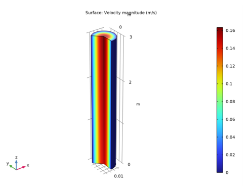
The velocity field is shown in Figure 1 and the temperature field in Figure 2. Both are plotted in a scaled view to get a clearer visualization of the results.
Figure 1: Velocity field.
Figure 2: Temperature field.
The comparison of the computed heat transfer coefficient with the Nusselt number correlations shows that the Local Nusselt number provides a good approximation over the whole cylinder. On the other hand, constant Nusselt number represents the region where velocity and temperature profile are fully developed (Figure 3).
Figure 3: Comparison of the computed heat transfer coefficient with the heat transfer coefficient estimation based onNusselt number correlations.
References
1. F.P. Incropera, D.P. DeWitt, T.L. Bergman, and A.S. Lavine, Fundamentals of Heat and Mass Transfer, 6th Edition, John Wiley & Sons, 2006.
2. A. Bejan et al., Heat Transfer Handbook, John Wiley & Sons, 2003.
Application Library path: Heat_Transfer_Module/Verification_Examples/circular_tube_nitf_laminar
Modeling Instructions
From the File menu, choose New.
New
In the New window, click  Model Wizard.
Model Wizard
1
In the Model Wizard window, click  2D Axisymmetric.
2
In the Select Physics tree, select Fluid Flow>Nonisothermal Flow>Laminar Flow.
3
Click Add.
4
Click  Study.
5
In the Select Study tree, select General Studies>Stationary.
6
Global Definitions
Parameters 1
1
In the Model Builder window, under Global Definitions click Parameters 1.
2
In the Settings window for Parameters, locate the Parameters section.
3
Definitions
Variables 1
Define several variables: A variable for the inlet velocity profile, a variable for the bulk temperature which is a radial weighted temperature, and similarly a variable for the bulk velocity. Finally, add variables to compare the simulation results with the literature values.
1
In the Model Builder window, under Component 1 (comp1) right-click Definitions and choose Variables.
2
In the Settings window for Variables, locate the Variables section.
3
Geometry 1
Rectangle 1 (r1)
1
In the Geometry toolbar, click  Rectangle.
2
In the Settings window for Rectangle, locate the Size and Shape section.
3
In the Width text field, type b/2.
4
In the Height text field, type L.
5
Click  Build All Objects.
Add Material
1
In the Home toolbar, click  Add Material to open the Add Material window.
2
Go to the Add Material window.
3
4
Click Add to Component in the window toolbar.
5
In the Home toolbar, click  Add Material to close the Add Material window.
Laminar Flow (spf)
Inlet 1
1
In the Model Builder window, under Component 1 (comp1) right-click Laminar Flow (spf) and choose Inlet.
2
3
In the Settings window for Inlet, locate the Velocity section.
4
In the U0 text field, type U.
Outlet 1
1
In the Physics toolbar, click  Boundaries and choose Outlet.
2
Heat Transfer in Fluids (ht)
In the Model Builder window, under Component 1 (comp1) click Heat Transfer in Fluids (ht).
Inflow 1
1
In the Physics toolbar, click  Boundaries and choose Inflow.
2
3
In the Settings window for Inflow, locate the Upstream Properties section.
4
In the Tustr text field, type T0.
Outflow 1
1
In the Physics toolbar, click  Boundaries and choose Outflow.
2
Heat Flux 1
1
In the Physics toolbar, click  Boundaries and choose Heat Flux.
2
3
In the Settings window for Heat Flux, locate the Heat Flux section.
4
In the q0 text field, type qw.
Mesh 1
Mapped 1
In the Mesh toolbar, click  Mapped.
Distribution 1
1
Right-click Mapped 1 and choose Distribution.
2
3
In the Settings window for Distribution, locate the Distribution section.
4
In the Number of elements text field, type 600.
Distribution 2
1
In the Model Builder window, right-click Mapped 1 and choose Distribution.
2
Click the  Zoom Extents button in the Graphics toolbar.
3
4
In the Settings window for Distribution, locate the Distribution section.
5
From the Distribution type list, choose Predefined.
6
In the Number of elements text field, type 33.
7
In the Element ratio text field, type 5.
8
Click  Build All.
Study 1
In the Home toolbar, click  Compute.
Results
Velocity, 3D (spf)
For better visualization of the results, use a scaled the view.
View 3D 2
In the Model Builder window, expand the Results>Views node.
Camera
1
In the Model Builder window, expand the View 3D 2 node, then click Camera.
2
In the Settings window for Camera, locate the Camera section.
3
From the View scale list, choose Manual.
4
In the z scale text field, type 0.1.
5
Click  Update.
6
Click the  Zoom Extents button in the Graphics toolbar.
Velocity, 3D (spf)
Click the  Zoom Extents button in the Graphics toolbar.
Heat transfer coefficient
1
In the Home toolbar, click  Add Plot Group and choose 1D Plot Group.
2
In the Settings window for 1D Plot Group, type Heat transfer coefficient in the Label text field.
Line Graph 1
1
Right-click Heat transfer coefficient and choose Line Graph.
2
3
In the Settings window for Line Graph, locate the y-Axis Data section.
4
In the Expression text field, type 4.36*ht.krr/b.
5
Locate the x-Axis Data section. From the Parameter list, choose Expression.
6
In the Expression text field, type z.
7
Click to expand the Legends section. Select the Show legends check box.
8
From the Legends list, choose Manual.
9
Line Graph 2
1
In the Model Builder window, right-click Heat transfer coefficient and choose Line Graph.
2
3
In the Settings window for Line Graph, locate the y-Axis Data section.
4
In the Expression text field, type Nu_D*ht.kmean/b.
5
Locate the x-Axis Data section. From the Parameter list, choose Expression.
6
In the Expression text field, type z.
7
Locate the Legends section. Select the Show legends check box.
8
From the Legends list, choose Manual.
9
Line Graph 3
1
Right-click Heat transfer coefficient and choose Line Graph.
2
3
In the Settings window for Line Graph, locate the y-Axis Data section.
4
In the Expression text field, type qw/(T-Tb).
5
Locate the x-Axis Data section. From the Parameter list, choose Expression.
6
In the Expression text field, type z.
7
Locate the Legends section. Select the Show legends check box.
8
From the Legends list, choose Manual.
9
Heat transfer coefficient
1
In the Model Builder window, click Heat transfer coefficient.
2
In the Heat transfer coefficient toolbar, click  Plot.