Convection Cooling of Circuit Boards — 3D Natural Convection

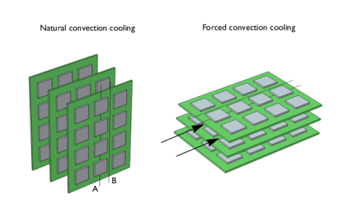
This example models the air cooling of circuit boards populated with multiple integrated circuits (ICs), which act as heat sources. Two possible cooling scenarios are shown in Figure 1: vertically aligned boards using natural convection, and horizontal boards with forced convection (fan cooling). In this case, contributions caused by the induced (forced) flow of air dominate the cooling. To achieve high accuracy, the simulation models heat transport in combination with the fluid flow.

Figure 1: Stacked circuit boards with multiple in-line heat sources. Line A represents the centerline of the row of ICs, and the area between lines A-B on the board represents the symmetry.

A common technique is to describe convective heat flux with a film-resistance coefficient, h. The heat-transfer equations then become simple to solve. However, this simplification requires that the coefficient is well determined which is difficult for many systems and conditions.

An alternative way to thoroughly describe the convective heat transfer is to model the heat transfer in combination with the fluid-flow field. The results then accurately describe the heat transport and temperature changes. From such simulations it is also possible to derive accurate estimations of the film coefficients. Such models are somewhat more complex but they are useful for unusual geometries and complex flows. The following example models the heat transfer of a circuit-board assembly using the Conjugate Heat Transfer predefined multiphysics coupling of the Heat Transfer Module. The modeled scenario is based on work published by A. Ortega (Ref. 1).

FR4 circuit board material (Ref. 2) and silicon are used as the solid materials composing the circuit board system. The model treats air properties as temperature dependent.

The dimensions of the original geometry are:

•

Board: length (in the flow direction) 130 mm, and the thickness is 2 mm

•

ICs: length and width are both 20 mm, and thickness is 2 mm

•

The boards are spaced 10 mm apart

Model Definition

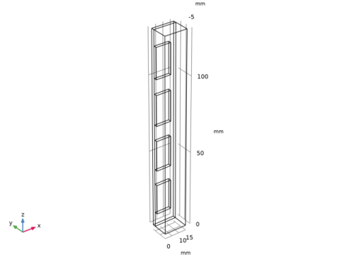
This example simulates natural convection cooling of a vertical circuit board as shown in Figure 1. Due to symmetry, it is sufficient to model a unit cell, from the back side of a board to the next back side, covering the area between lines A and B in Figure 1. Figure 2 depicts the three-dimensional geometry.

Figure 2: The modeled geometry.

The model makes use of the Conjugate Heat Transfer predefined multiphysics coupling with a stationary study to set up the simulation. The heat rate per unit volume is 1.25 MW/m3. Due to heating of the fluid, deviations occur in the local density, ρ, compared to the inlet density, ρref. This results in a local buoyancy force defined using the feature in the interface.

Results and Discussion

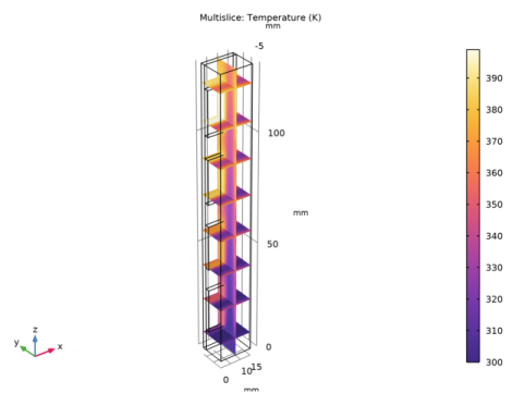
The temperature distribution is shown on Figure 3. The temperature increase at the hottest spot of each component computed in this 3D model is approximately two degrees higher than that for the 2D model (see Convection Cooling of Circuit Boards — 2D Natural Convection for 2D model description and results). In addition, the temperature difference among the various ICs is smaller in the 3D model, which predicts a more uniform temperature rise of the ICs. The ICs have an operating temperature between 50 K and 100 K above ambient. This result is closer to reality compared to the 2D simulation because it also includes the horizontal gaps between the ICs.

Figure 3: Temperature distribution for 3D model

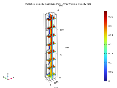
The difference in temperature rise along the board’s height is explained primarily by the fluid-flow pattern (Figure 4). The maximum fluid velocity is slightly higher for the 3D case than for the 2D case. More importantly, the flow field behaves differently in the 3D case. When making a comparison between the 2D and 3D models, it can be noticed that the velocity fields are rather similar along the centerline of the heat sources. However, there is a channeling effect from the horizontal gaps.

Figure 4: Velocity field distribution.

References

1. A. Ortega, “Air Cooling of Electronics: A Personal Perspective 1981-2001,” presentation material, IEEE SMITHERM Symposium, 2002.

2. C. Bailey, “Modeling the Effect of Temperature on Product Reliability,” Proc. 19th IEEE SMITHERM Symposium, 2003.

Heat_Transfer_Module/Power_Electronics_and_Electronic_Cooling/circuit_board_nat_3d

Modeling Instructions

From the menu, choose .

New

In the window, click

Model Wizard

In the window, click

In the tree, select .

Click .

Click

In the tree, select .

Click

Global Definitions

Parameters 1

In the window, under click .

In the window for , locate the section.

In the table, enter the following settings:


Name	Expression	Value	Description
q_source	1[W]/(20202[mm^3])	1.25E6 W/m³	Heating power per unit volume
T0	300[K]	300 K	External air temperature
patm	1[atm]	1.0133E5 Pa	Air pressure