PDF

Convection Cooling of Circuit Boards — 2D Natural Convection
Introduction
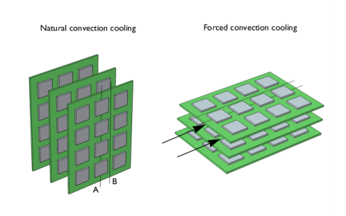
This example models the air cooling of circuit boards populated with multiple integrated circuits (ICs), which act as heat sources. Two possible cooling scenarios are shown in Figure 1: vertically aligned boards using natural convection, and horizontal boards with forced convection (fan cooling). In this case, contributions caused by the induced (forced) flow of air dominate the cooling. To achieve high accuracy, the simulation models heat transport in combination with the fluid flow.
Figure 1: Stacked circuit boards with multiple in-line heat sources. Line A represents the centerline of the row of ICs, and the area between lines A-B on the board represents the symmetry.
A common technique is to describe convective heat flux with a film-resistance coefficient, h. The heat-transfer equations then become simple to solve. However, this simplification requires that the coefficient is well determined which is difficult for many systems and conditions.
An alternative way to thoroughly describe the convective heat transfer is to model the heat transfer in combination with the fluid-flow field. The results then accurately describe the heat transport and temperature changes. From such simulations it is also possible to derive accurate estimations of the film coefficients. Such models are somewhat more complex but they are useful for unusual geometries and complex flows. The following example models the heat transfer of a circuit-board assembly using the Conjugate Heat Transfer predefined multiphysics coupling of the Heat Transfer Module. The modeled scenario is based on work published by A. Ortega (Ref. 1).
FR4 circuit board material (Ref. 2) and silicon are used as the solid materials composing the circuit board system. The model treats air properties as temperature dependent.
The dimensions of the original geometry are:
Board: length (in the flow direction) 130 mm, and the thickness is 2 mm
ICs: length and width are both 20 mm, and thickness is 2 mm
Model Definition
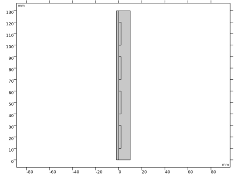
This example models the natural convection. The simplified model considers the 2D cross section, from the board’s back side to the next board’s back side, through the center of a row of ICs (as indicated by line A in Figure 1). Figure 2 depicts the 2D geometry.
Figure 2: The modeled geometry in 2D.
The model makes use of the Conjugate Heat Transfer predefined multiphysics coupling with a stationary study to set up the simulation. The heating rate per unit volume in the solid is 0.83 MW/m3. It is 2/3 of the real heat power in order to represent the lateral average heating power (that is, taking into account the open slots between the ICs).
Due to heating of the fluid, deviations occur in the local density, ρ, compared to the inlet density, ρ0. This results in a local buoyancy force defined using the Gravity feature in the Single Phase Flow interface.
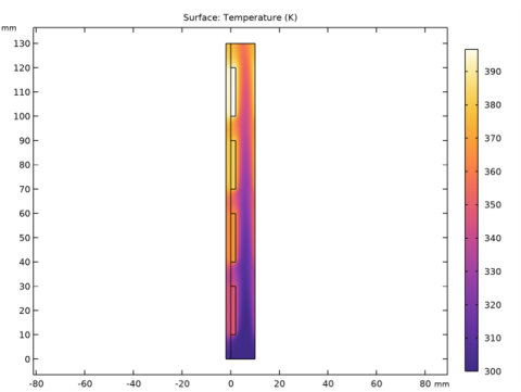
Figure 3: Temperature distribution.
Boundary Conditions
The top and bottom boundaries are open boundaries with given external air temperature. In addition, no slip conditions at the surfaces of the board and the ICs are applied. You should also set the lateral boundaries periodic with respect to temperature, making the temperatures equal on both boundaries at every value. Finally, the models apply continuity of temperature and heat flux at all interior boundaries.
Results and Discussion
The results (Figure 3) show that the temperature of the ICs (the heat sources) increases considerably under a constant heating load from the components. Note that the temperature increase of the sources varies from 50 K for the lowest IC up to 100 K at the top IC. This is a result of the thermal “footprint” of the heat sources. Another interesting result is that the circuit board contributes a large amount of cooling power on its back side, although the thermal conductivity is quite small. This is apparent in the result plots as a temperature rise in the fluid at the right-hand boundary (that is, the back side of the next board in the stack).
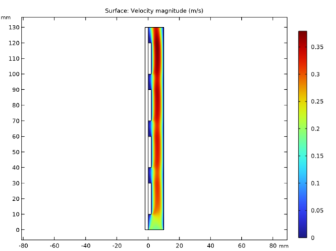
Figure 4: Velocity field.
References
1. A. Ortega, “Air Cooling of Electronics: A Personal Perspective 1981-2001,” presentation material, IEEE SMITHERM Symposium, 2002.
2. C. Bailey, “Modeling the Effect of Temperature on Product Reliability,” Proc. 19th IEEE SMITHERM Symposium, 2003.
Application Library path: Heat_Transfer_Module/Power_Electronics_and_Electronic_Cooling/circuit_board_nat_2d
Modeling Instructions
From the File menu, choose New.
New
In the New window, click  Model Wizard.
Model Wizard
1
In the Model Wizard window, click  2D.
2
In the Select Physics tree, select Heat Transfer>Conjugate Heat Transfer>Laminar Flow.
3
Click Add.
4
Click  Study.
5
In the Select Study tree, select General Studies>Stationary.
6
Global Definitions
Parameters 1
1
In the Model Builder window, under Global Definitions click Parameters 1.
2
In the Settings window for Parameters, locate the Parameters section.
3
Geometry 1
1
In the Model Builder window, under Component 1 (comp1) click Geometry 1.
2
In the Settings window for Geometry, locate the Units section.
3
From the Length unit list, choose mm.
Rectangle 1 (r1)
1
In the Geometry toolbar, click  Rectangle.
2
In the Settings window for Rectangle, locate the Size and Shape section.
3
In the Width text field, type 12.
4
In the Height text field, type 130.
5
Locate the Position section. In the x text field, type -2.
6
Click to expand the Layers section. Select the Layers to the left check box.
7
Clear the Layers on bottom check box.
8
9
In the Geometry toolbar, click  Build All.
Rectangle 2 (r2)
1
In the Geometry toolbar, click  Rectangle.
2
In the Settings window for Rectangle, locate the Size and Shape section.
3
In the Width text field, type 2.
4
In the Height text field, type 20.
5
Locate the Position section. In the y text field, type 10.
6
In the Geometry toolbar, click  Build All.
Array 1 (arr1)
1
In the Geometry toolbar, click  Transforms and choose Array.
2
3
In the Settings window for Array, locate the Size section.
4
In the y size text field, type 4.
5
Locate the Displacement section. In the y text field, type 30.
6
In the Geometry toolbar, click  Build All.
The geometry should now look like that in Figure 2.
Definitions
IC
1
In the Definitions toolbar, click  Explicit.
2
In the Settings window for Explicit, type IC in the Label text field.
3
Add Material
1
In the Home toolbar, click  Add Material to open the Add Material window.
2
Go to the Add Material window.
3
4
Click Add to Component in the window toolbar.
5
In the tree, select Built-in>Silicon.
6
Click Add to Component in the window toolbar.
7
In the tree, select Built-in>FR4 (Circuit Board).
8
Click Add to Component in the window toolbar.
9
In the Home toolbar, click  Add Material to close the Add Material window.
Materials
Air (mat1)
1
In the Model Builder window, under Component 1 (comp1)>Materials click Air (mat1).
2
3
In the Settings window for Material, locate the Geometric Entity Selection section.
4
Click  Create Selection.
5
In the Create Selection dialog box, type Air in the Selection name text field.
6
Silicon (mat2)
1
In the Model Builder window, click Silicon (mat2).
2
In the Settings window for Material, locate the Geometric Entity Selection section.
3
From the Selection list, choose IC.
FR4 (Circuit Board) (mat3)
1
In the Model Builder window, click FR4 (Circuit Board) (mat3).
2
Laminar Flow (spf)
1
In the Model Builder window, under Component 1 (comp1) click Laminar Flow (spf).
2
In the Settings window for Laminar Flow, locate the Domain Selection section.
3
From the Selection list, choose Air.
4
Locate the Physical Model section. Select the Include gravity check box.
Open Boundary 1
1
In the Physics toolbar, click  Boundaries and choose Open Boundary.
2
Heat Transfer in Solids and Fluids (ht)
1
In the Model Builder window, under Component 1 (comp1) click Heat Transfer in Solids and Fluids (ht).
2
In the Settings window for Heat Transfer in Solids and Fluids, locate the Physical Model section.
3
In the Tref text field, type T0.
Fluid 1
1
In the Model Builder window, under Component 1 (comp1)>Heat Transfer in Solids and Fluids (ht) click Fluid 1.
2
In the Settings window for Fluid, locate the Domain Selection section.
3
From the Selection list, choose Air.
Open Boundary 1
1
In the Physics toolbar, click  Boundaries and choose Open Boundary.
2
3
In the Settings window for Open Boundary, locate the Upstream Properties section.
4
In the Tustr text field, type T0.
Heat Source 1
1
In the Physics toolbar, click  Domains and choose Heat Source.
2
In the Settings window for Heat Source, locate the Domain Selection section.
3
From the Selection list, choose IC.
4
Locate the Heat Source section. In the Q0 text field, type q_source.
Periodic Condition 1
1
In the Physics toolbar, click  Boundaries and choose Periodic Condition.
2
Study 1
In the Home toolbar, click  Compute.
Results
Temperature (ht)
The first default plot shows the temperature distribution as in Figure 3.
Velocity (spf)
This default plot shows the velocity magnitude as in Figure 4.