PDF

Heat Generation in a Disc Brake
Introduction
Cars need brakes for obvious reasons, and you do not want these to fail. Brake failure can be caused by many things, one of which is the overheating of the brake’s disc. This example models the heat generation and dissipation in a disc brake of an ordinary car during panic braking and the following release period. When the driver is pressing down on the brakes, kinetic energy is transformed into thermal energy. If the brake discs overheat, temperature overload can change the material properties of the brake causing it to fade. Braking power already starts to fade at temperatures above 600 K. This is why it is so important during the design-stages to simulate the transient heating and convective cooling to figure out what the minimum interval between a series of brake engagements is.
In this application, an 1,800 kg car is traveling at 25 m/s (90 km/h or about 56 mph), until the driver suddenly panic brakes for 2 seconds. At that point the eight brake pads slow the car down at a rate of 10 m/s2 (assuming the wheels do not skid against the road). Upon braking for two seconds the driver releases the brake, leaving the car traveling at 5 m/s for eight seconds without engaging the brakes. The questions to analyze with the model are:
Model Definition
Model the brake disc as a 3D solid with shape and dimensions as in Figure 1. The disc has a radius of 0.14 m and a thickness of 0.013 m.
Figure 1: Model geometry, including disc and pad.
The model also includes heat conduction in the disc and the pad through the transient heat transfer equation. The heat dissipation from the disc and pad surfaces to the surrounding air is described by both convection and radiation. Table 1 summarizes the thermal properties of the materials used in this application (Ref. 1).
ρ (kg/m3)
Cp (J/(kg·K))
k (W/(m·K))
ε
After 2 s, contact is made at the interface between the disc and the pad. Neglecting drag and other losses outside the brakes, the brakes’ retardation power is given by the negative of the time derivative of the car’s kinetic energy:
Here m is the car’s mass (1800 kg) and v denotes its speed. Figure 2 shows the profile of v and Figure 3 shows the corresponding acceleration profile.
Figure 2: Velocity profile of the disc.
Figure 3: Acceleration profile of the disc.
At one of the eight brakes, the frictional heat source is:
The contact pressure between the disc and the pad is related to the frictional heat source per unit area, Qb=Pb/A, according to:
where the friction coefficient μ is here equal to 0.3.
The disc and pad dissipate the heat produced at the boundary between the brake pad and the disc by convection and radiation. This example models the rotation as convection in the disc. The local disc velocity vector is
At the end of the computation, produced and dissipated heat can be recovered using the relations
(1)
Results and Discussion
The surface temperatures of the disc and the pad vary with both time and position. At the contact surface between the pad and the disc the temperature increases when the brake is engaged and then decreases again as the brake is released. You can best see these results in COMSOL Multiphysics by generating an animation. Figure 4 displays the surface temperatures just before the end of the braking. A “hotspot” is visible at the contact between the brake pad and disc, just at the pad’s edge. This is the area that could overheat to the point of brake failure or fade. The figure also shows the temperature decreasing along the rotational trace after the pad. During the rest, the temperature becomes significantly lower and more uniform in the disc and the pad.
Figure 4: Surface temperature of the brake disc and pad just before releasing the brake (t = 3.8 s).
To investigate the position of the hotspot and the time of the temperature maximum, it is helpful to plot temperature versus time along the line from the center to the pad’s edge shown in Figure 5. The result is displayed in Figure 6. You can see that the maximum temperature is approximately 430 K. The hotspot is positioned close to the radially outer edge of the pad. The highest temperature occurs approximately 1 s after engaging the brake.
Figure 5: The radial line probed in the temperature vs. time plot in Figure 6.
Figure 6: Temperature profile along the line indicated in Figure 5 at the disc surface (z = 0.013 m) as a function of time.
To investigate how much of the generated heat is dissipated to the air, study the surface integrals of the produced heat and the dissipated heat. These integrals give the total heat rate (W) for heat production, Qprod, and heat dissipation, Qdiss, as functions of time for the brake disc. The time integrals of these two quantities, Wprod and Wdiss, give the total heat (J) produced and dissipated, respectively, in the brake disc. Figure 7 shows a plot of the total produced heat and dissipated heat versus time. Eight seconds after the driver has stopped braking, a mere fraction of the produced heat has been dissipated. In other words, in order to cool down the system sufficiently the brake needs to remain disengaged for a much longer period than these eight seconds (100 seconds, in fact).
Figure 7: Comparison of total produced heat (solid line) and dissipated heat (dashed).
The results of this application can help engineers investigate how much abuse, in terms of specific braking sequences, a certain brake-disc design can tolerate before overheating. It is also possible to modify the parameters affecting the heat dissipation and investigate their influence.
Reference
1. J.M. Coulson and J.F. Richardson, Chemical Engineering, vol. 1, eq. 9.88; material properties from appendix A2.
Application Library path: Heat_Transfer_Module/Thermal_Contact_and_Friction/brake_disc
Modeling Instructions
From the File menu, choose New.
New
In the New window, click  Model Wizard.
Model Wizard
1
In the Model Wizard window, click  3D.
2
In the Select Physics tree, select Heat Transfer>Heat Transfer in Solids (ht).
3
Click Add.
4
Click  Study.
5
In the Select Study tree, select General Studies>Time Dependent.
6
Geometry 1
Define the global parameters by loading the corresponding text file provided.
Global Definitions
Parameters 1
1
In the Model Builder window, under Global Definitions click Parameters 1.
2
In the Settings window for Parameters, locate the Parameters section.
3
Click  Load from File.
4
Geometry 1
Cylinder 1 (cyl1)
1
In the Geometry toolbar, click  Cylinder.
2
In the Settings window for Cylinder, locate the Size and Shape section.
3
In the Radius text field, type 0.14.
4
In the Height text field, type 0.013.
5
In the Geometry toolbar, click  Build All.
Cylinder 2 (cyl2)
1
In the Geometry toolbar, click  Cylinder.
2
In the Settings window for Cylinder, locate the Size and Shape section.
3
In the Radius text field, type 0.08.
4
In the Height text field, type 0.01.
5
Locate the Position section. In the z text field, type 0.013.
6
In the Geometry toolbar, click  Build All.
Work Plane 1 (wp1)
1
In the Geometry toolbar, click  Work Plane.
2
In the Settings window for Work Plane, locate the Plane Definition section.
3
In the z-coordinate text field, type 0.013.
4
Click  Show Work Plane.
Work Plane 1 (wp1)>Cubic Bézier 1 (cb1)
1
In the Work Plane toolbar, click  More Primitives and choose Cubic Bézier.
2
In the Settings window for Cubic Bézier, locate the Control Points section.
3
In row 1, set yw to 0.135.
4
In row 2, set xw to 0.02, and yw to 0.135.
5
In row 3, set xw to 0.05, and yw to 0.13.
6
In row 4, set xw to 0.04, and yw to 0.105.
7
Locate the Weights section. In the 3 text field, type 2.5.
Work Plane 1 (wp1)>Cubic Bézier 2 (cb2)
1
In the Work Plane toolbar, click  More Primitives and choose Cubic Bézier.
2
In the Settings window for Cubic Bézier, locate the Control Points section.
3
In row 1, set xw to 0.04.
4
In row 1, set yw to 0.105, and yw to 0.03., and yw to 0.08.
5
In row 3, set xw to 0.035, and yw to 0.09., and yw to 0.09.
Work Plane 1 (wp1)>Cubic Bézier 3 (cb3)
1
In the Work Plane toolbar, click  More Primitives and choose Cubic Bézier.
2
In the Settings window for Cubic Bézier, locate the Control Points section.
3
In row 1, set yw to 0.09.
4
In row 2, set xw to -0.035, and yw to 0.09.
5
In row 3, set xw to -0.03, and yw to 0.08.
6
In row 4, set xw to -0.04, and yw to 0.105.
Work Plane 1 (wp1)>Cubic Bézier 4 (cb4)
1
In the Work Plane toolbar, click  More Primitives and choose Cubic Bézier.
2
In the Settings window for Cubic Bézier, locate the Control Points section.
3
In row 1, set xw to -0.04.
4
In row 2, set xw to -0.05, and yw to 0.09., and yw to 0.13.
5
In row 3, set xw to -0.02, and yw to 0.135.
6
In row 4, set yw to 0.135.
7
Locate the Weights section. In the 2 text field, type 2.5.
8
In the Work Plane toolbar, click  Build All.
Work Plane 1 (wp1)>Convert to Solid 1 (csol1)
1
In the Work Plane toolbar, click  Conversions and choose Convert to Solid.
2
Click in the Graphics window and then press Ctrl+A to select all objects.
3
In the Work Plane toolbar, click  Build All.
Extrude 1 (ext1)
1
In the Model Builder window, under Component 1 (comp1)>Geometry 1 right-click Work Plane 1 (wp1) and choose Extrude.
2
In the Settings window for Extrude, locate the Distances section.
3
4
In the Geometry toolbar, click  Build All.
The model geometry is now complete.
Next, define some selections of certain boundaries. You will use them when defining the settings for component couplings, boundary conditions, and so on.
Definitions
Disc Faces
1
In the Definitions toolbar, click  Explicit.
2
In the Settings window for Explicit, type Disc Faces in the Label text field.
3
Locate the Input Entities section. From the Geometric entity level list, choose Boundary.
4
Pad Faces
1
In the Definitions toolbar, click  Explicit.
2
In the Settings window for Explicit, type Pad Faces in the Label text field.
3
Locate the Input Entities section. From the Geometric entity level list, choose Boundary.
4
Contact Faces
1
In the Definitions toolbar, click  Explicit.
2
In the Settings window for Explicit, type Contact Faces in the Label text field.
3
Locate the Input Entities section. From the Geometric entity level list, choose Boundary.
To select the contact surface boundary, it is convenient to temporarily switch to wireframe rendering.
4
Click the  Wireframe Rendering button in the Graphics toolbar.
5
6
Click the  Wireframe Rendering button in the Graphics toolbar again to return to the original state.
External Surfaces
1
In the Definitions toolbar, click  Explicit.
2
In the Settings window for Explicit, type External Surfaces in the Label text field.
3
Locate the Input Entities section. Select the All domains check box.
4
Locate the Output Entities section. From the Output entities list, choose Adjacent boundaries.
These instructions make you select the external boundaries of the wheel and the pad.
Integration 1 (intop1)
1
In the Definitions toolbar, click  Nonlocal Couplings and choose Integration.
2
In the Settings window for Integration, locate the Source Selection section.
3
From the Geometric entity level list, choose Boundary.
4
From the Selection list, choose Contact Faces.
Integration 2 (intop2)
1
In the Definitions toolbar, click  Nonlocal Couplings and choose Integration.
2
In the Settings window for Integration, locate the Source Selection section.
3
From the Geometric entity level list, choose Boundary.
4
From the Selection list, choose External Surfaces.
Now, define the velocity and acceleration of the car through these two piecewise and analytic functions.
Piecewise 1 (pw1)
1
In the Definitions toolbar, click  Piecewise.
2
In the Settings window for Piecewise, type v in the Function name text field.
3
Locate the Definition section. In the Argument text field, type t.
4
From the Smoothing list, choose Continuous second derivative.
5
From the Transition zone list, choose Absolute size.
6
In the Size of transition zone text field, type 0.2.
The function definition expects nondimensional quantities for the interval bounds, and the function values. The function definition below uses unit conversions to do so.
7
Find the Intervals subsection. In the table, enter the following settings:
8
Locate the Units section. In the Arguments text field, type s.
9
In the Function text field, type m/s.
10
Analytic 1 (an1)
1
In the Definitions toolbar, click  Analytic.
2
In the Settings window for Analytic, type a in the Function name text field.
3
Locate the Definition section. In the Expression text field, type d(v(t),t).
4
In the Arguments text field, type t.
5
Locate the Units section. In the table, enter the following settings:
6
In the Function text field, type m/s^2.
7
Locate the Plot Parameters section. In the table, enter the following settings:
8
Materials
Disc
1
In the Materials toolbar, click  Blank Material.
2
In the Settings window for Material, type Disc in the Label text field.
3
Locate the Material Contents section. In the table, enter the following settings:
Pad
1
In the Materials toolbar, click  Blank Material.
2
In the Settings window for Material, type Pad in the Label text field.
3
4
Locate the Material Contents section. In the table, enter the following settings:
Heat Transfer in Solids (ht)
Solid 1
In the Model Builder window, under Component 1 (comp1)>Heat Transfer in Solids (ht) click Solid 1.
Translational Motion 1
1
In the Physics toolbar, click  Attributes and choose Translational Motion.
2
3
In the Settings window for Translational Motion, locate the Translational Motion section.
4
Specify the utrans vector as
Heat Flux 1
1
In the Physics toolbar, click  Boundaries and choose Heat Flux.
2
In the Settings window for Heat Flux, locate the Boundary Selection section.
3
From the Selection list, choose All boundaries.
4
Locate the Heat Flux section. From the Flux type list, choose Convective heat flux.
5
From the Heat transfer coefficient list, choose External forced convection.
6
In the L text field, type 0.14.
7
In the U text field, type v(t).
8
In the Text text field, type T_air.
Thermal Contact 1
1
In the Physics toolbar, click  Boundaries and choose Thermal Contact.
2
3
In the Settings window for Thermal Contact, locate the Contact Surface Properties section.
4
In the p text field, type ht.tc1.Qb/(mu*v(t)).
5
In the Hc text field, type 800[MPa].
6
Locate the Thermal Friction section. Click the Heat rate button.
7
In the Pb text field, type -m_car*v(t)*a(t)/8.
Initial Values 1
1
In the Model Builder window, click Initial Values 1.
2
In the Settings window for Initial Values, locate the Initial Values section.
3
In the T text field, type T_air.
Surface-to-Ambient Radiation 1
1
In the Physics toolbar, click  Boundaries and choose Surface-to-Ambient Radiation.
2
In the Settings window for Surface-to-Ambient Radiation, locate the Boundary Selection section.
3
From the Selection list, choose Disc Faces.
4
Locate the Surface-to-Ambient Radiation section. From the ε list, choose User defined. In the associated text field, type 0.28.
5
In the Tamb text field, type T_air.
Surface-to-Ambient Radiation 2
1
In the Physics toolbar, click  Boundaries and choose Surface-to-Ambient Radiation.
2
In the Settings window for Surface-to-Ambient Radiation, locate the Boundary Selection section.
3
From the Selection list, choose Pad Faces.
4
Locate the Surface-to-Ambient Radiation section. From the ε list, choose User defined. In the associated text field, type 0.8.
5
In the Tamb text field, type T_air.
Symmetry 1
1
In the Physics toolbar, click  Boundaries and choose Symmetry.
2
To compute the produced and dissipated heats, integrate the corresponding heat rate variables, Q_prod and Q_diss, over time. For this purpose, define two ODEs using a Global Equations node.
3
Click the  Show More Options button in the Model Builder toolbar.
4
In the Show More Options dialog box, in the tree, select the check box for the node Physics>Equation-Based Contributions.
5
Global Equations 1
1
In the Physics toolbar, click  Global and choose Global Equations.
2
In the Settings window for Global Equations, locate the Units section.
3
Click  Select Dependent Variable Quantity.
4
In the Physical Quantity dialog box, type energy in the text field.
5
Click  Filter.
6
In the tree, select General>Energy (J).
7
8
In the Settings window for Global Equations, locate the Units section.
9
Click  Select Source Term Quantity.
10
In the Physical Quantity dialog box, type power in the text field.
11
Click  Filter.
12
In the tree, select General>Power (W).
13
14
In the Settings window for Global Equations, locate the Global Equations section.
15
Here, W_prodt (resp. W_disst) is COMSOL Multiphysics syntax for the time derivative of W_prod (resp. W_diss). The quantities intop1(ht.tc1.Qb) and intop2(ht.q0+ht.rflux) correspond to Q_prod and Q_diss. The table thus defines the first-order ODEs corresponding to Equation 1, so that W_prod and W_diss host the produced and dissipated heats. The initial values follow from setting t = 0.
Mesh 1
Free Triangular 1
1
In the Mesh toolbar, click  Boundary and choose Free Triangular.
2
Click the  Transparency button in the Graphics toolbar.
3
4
Click the  Transparency button in the Graphics toolbar again to return to the original state.
Size
1
In the Model Builder window, click Size.
2
In the Settings window for Size, locate the Element Size section.
3
From the Predefined list, choose Extra fine.
Swept 1
In the Mesh toolbar, click  Swept.
Distribution 1
1
Right-click Swept 1 and choose Distribution.
2
In the Settings window for Distribution, locate the Distribution section.
3
In the Number of elements text field, type 2.
4
In the Model Builder window, right-click Mesh 1 and choose Build All.
The complete mesh consists of roughly 5800 elements.
Study 1
Step 1: Time Dependent
1
In the Model Builder window, under Study 1 click Step 1: Time Dependent.
2
In the Settings window for Time Dependent, locate the Study Settings section.
3
In the Output times text field, type range(0,0.5,1.5) range(1.55,0.05,3) range(3.2,0.2,5) range(6,1,12).
Solution 1 (sol1)
1
In the Study toolbar, click  Show Default Solver.
2
In the Model Builder window, expand the Solution 1 (sol1) node, then click Time-Dependent Solver 1.
3
In the Settings window for Time-Dependent Solver, click to expand the Time Stepping section.
4
From the Steps taken by solver list, choose Intermediate.
This setting forces the solver to take at least one step in each specified interval.
5
In the Study toolbar, click  Compute.
Results
The first of the two default plots displays the surface temperature of the brake disc and pad at the end of the simulation interval. Modify this plot to show the time step just before releasing the brake.
Temperature (ht)
1
In the Model Builder window, under Results click Temperature (ht).
2
In the Settings window for 3D Plot Group, locate the Data section.
3
From the Time (s) list, choose 3.8.
Surface 2
1
In the Model Builder window, expand the Temperature (ht) node, then click Surface 2.
2
In the Settings window for Surface, click to expand the Title section.
3
From the Title type list, choose None.
Surface 3
1
In the Model Builder window, click Surface 3.
2
In the Settings window for Surface, locate the Title section.
3
From the Title type list, choose None.
4
In the Temperature (ht) toolbar, click  Plot.
Compare the result to the plot shown in Figure 4.
To compare the total produced heat and the dissipated heat, as done in Figure 7, follow the steps given below.
Dissipated and Produced Heats
1
In the Home toolbar, click  Add Plot Group and choose 1D Plot Group.
2
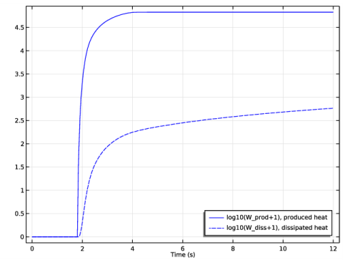
In the Settings window for 1D Plot Group, type Dissipated and Produced Heats in the Label text field.
3
Click to expand the Title section. From the Title type list, choose None.
4
Click to collapse the Title section. Locate the Plot Settings section. Select the x-axis label check box.
5
6
Locate the Legend section. From the Position list, choose Lower right.
Point Graph 1
1
In the Dissipated and Produced Heats toolbar, click  Point Graph.
2
3
In the Settings window for Point Graph, locate the y-Axis Data section.
4
In the Expression text field, type log10(W_prod+1).
5
Click to expand the Coloring and Style section. From the Color list, choose Blue.
6
Click to expand the Legends section. Select the Show legends check box.
7
From the Legends list, choose Manual.
8
Point Graph 2
1
Right-click Point Graph 1 and choose Duplicate.
2
In the Settings window for Point Graph, locate the y-Axis Data section.
3
In the Expression text field, type log10(W_diss+1).
4
Locate the Coloring and Style section. Find the Line style subsection. From the Line list, choose Dashed.
5
Locate the Legends section. In the table, enter the following settings:
Dissipated and Produced Heats
Finally, follow the steps below to reproduce the plot in Figure 6.
Cut Line 3D 1
1
In the Results toolbar, click  Cut Line 3D.
2
In the Settings window for Cut Line 3D, locate the Line Data section.
3
In row Point 1, set Z to 0.013.
4
In row Point 2, set X to -0.047, y to 0.1316, and z to 0.013.
5
Parametric Extrusion 1D 1
1
In the Results toolbar, click  More Datasets and choose Parametric Extrusion 1D.
2
In the Settings window for Parametric Extrusion 1D, locate the Data section.
3
From the Time selection list, choose From list.
4
Temperature Profile vs. Time
1
In the Results toolbar, click  2D Plot Group.
2
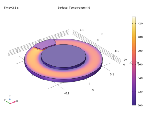
In the Settings window for 2D Plot Group, type Temperature Profile vs. Time in the Label text field.
Surface 1
1
In the Temperature Profile vs. Time toolbar, click  Surface.
2
In the Settings window for Surface, locate the Coloring and Style section.
3
From the Color table list, choose HeatCameraLight.
Height Expression 1
1
In the Temperature Profile vs. Time toolbar, click  Height Expression.
2
In order to visualize the temperature on each side of the thermal contact, follow the next steps.
Temperature (ht) 1
In the Model Builder window, right-click Temperature (ht) and choose Duplicate.
Surface 2
1
In the Model Builder window, expand the Results>Temperature (ht) node.
2
Right-click Results>Temperature (ht)>Surface 2 and choose Delete.
Surface 3
In the Model Builder window, right-click Surface 3 and choose Delete.
Surface 2
1
In the Model Builder window, expand the Results>Temperature (ht) 1 node, then click Surface 2.
2
In the Settings window for Surface, click to expand the Inherit Style section.
3
From the Plot list, choose None.
Surface 1
In the Model Builder window, under Results>Temperature (ht) 1 right-click Surface 1 and choose Delete.
Contact temperatures (ht)
1
In the Model Builder window, under Results click Temperature (ht) 1.
2
In the Settings window for 3D Plot Group, type Contact temperatures (ht) in the Label text field.
Upside
1
In the Model Builder window, under Results>Contact temperatures (ht) click Surface 2.
2
In the Settings window for Surface, type Upside in the Label text field.
3
Locate the Expression section. Select the Description check box.
4
5
Locate the Coloring and Style section. From the Color table list, choose HeatCameraLight.
Downside
1
In the Model Builder window, under Results>Contact temperatures (ht) click Surface 3.
2
In the Settings window for Surface, type Downside in the Label text field.
3
Locate the Expression section. Select the Description check box.
4
Deformation
1
In the Model Builder window, expand the Upside node, then click Deformation.
2
In the Settings window for Deformation, locate the Scale section.
3
In the Scale factor text field, type 10.
4
In the Contact temperatures (ht) toolbar, click  Plot.