|
|
|
|
•
|
|
•
|
|
•
|
|
1
|
|
2
|
|
3
|
Click Add.
|
|
4
|
In the Select Physics tree, select Fluid Flow>Porous Media and Subsurface Flow>Free and Porous Media Flow (fp).
|
|
5
|
Click Add.
|
|
6
|
|
7
|
In the Velocity field components table, enter the following settings:
|
|
8
|
|
9
|
In the Select Physics tree, select Fluid Flow>Porous Media and Subsurface Flow>Free and Porous Media Flow (fp).
|
|
10
|
Click Add.
|
|
11
|
|
12
|
In the Velocity field components table, enter the following settings:
|
|
13
|
|
14
|
Click
|
|
15
|
In the Select Study tree, select Preset Studies for Selected Physics Interfaces>Hydrogen Fuel Cell>Stationary with Initialization.
|
|
16
|
Click
|
|
1
|
|
2
|
|
3
|
|
4
|
Browse to the model’s Application Libraries folder and double-click the file sofc_unit_cell_parameters.txt.
|
|
1
|
|
2
|
|
3
|
|
4
|
|
1
|
|
2
|
|
3
|
|
4
|
|
5
|
|
6
|
|
1
|
|
2
|
|
3
|
|
4
|
|
5
|
|
6
|
|
1
|
|
2
|
|
3
|
|
4
|
|
5
|
|
6
|
|
1
|
|
2
|
|
3
|
|
4
|
|
5
|
|
6
|
|
7
|
|
1
|
|
2
|
|
3
|
|
4
|
|
5
|
|
6
|
|
7
|
|
8
|
|
1
|
In the Model Builder window, under Component 1 (comp1)>Geometry 1 right-click Work Plane 1 (wp1) and choose Extrude.
|
|
2
|
|
4
|
|
5
|
|
1
|
|
2
|
|
1
|
|
2
|
|
1
|
|
2
|
|
1
|
|
2
|
|
1
|
|
2
|
|
1
|
|
2
|
In the Settings window for Free and Porous Media Flow, type Free and Porous Media Flow - Cathode in the Label text field.
|
|
3
|
|
4
|
|
1
|
|
2
|
In the Settings window for Free and Porous Media Flow, type Free and Porous Media Flow - Anode in the Label text field.
|
|
3
|
|
4
|
|
1
|
|
2
|
|
3
|
|
1
|
|
2
|
|
3
|
Select the H2O check box.
|
|
1
|
|
2
|
|
3
|
|
1
|
|
2
|
|
3
|
|
1
|
|
2
|
|
3
|
|
1
|
|
2
|
|
3
|
|
1
|
|
2
|
|
3
|
|
1
|
|
2
|
|
3
|
In the tree, select Fuel Cell and Electrolyzer>Solid Oxides>Yttria-Stabilized Zirconia, 8YSZ, (ZrO2)0.92-(Y2O3)0.08.
|
|
4
|
|
5
|
|
1
|
In the Settings window for H2 Gas Diffusion Electrode, locate the Electrode Charge Transport section.
|
|
2
|
|
3
|
Locate the Effective Electrolyte Charge Transport section. From the Effective conductivity correction list, choose User defined. In the fl text field, type fl_a.
|
|
4
|
|
1
|
|
2
|
In the Settings window for H2 Gas Diffusion Electrode Reaction, click to expand the Reference Pressures section.
|
|
3
|
|
4
|
|
5
|
|
6
|
|
1
|
In the Model Builder window, under Component 1 (comp1)>Hydrogen Fuel Cell (fc) click O2 Gas Diffusion Electrode 1.
|
|
2
|
In the Settings window for O2 Gas Diffusion Electrode, locate the Electrode Charge Transport section.
|
|
3
|
|
4
|
Locate the Effective Electrolyte Charge Transport section. From the Effective conductivity correction list, choose User defined. In the fl text field, type fl_c.
|
|
5
|
|
1
|
|
2
|
In the Settings window for O2 Gas Diffusion Electrode Reaction, click to expand the Reference Pressures section.
|
|
3
|
|
4
|
|
5
|
|
1
|
|
1
|
|
3
|
|
4
|
|
1
|
In the Model Builder window, expand the Component 1 (comp1)>Hydrogen Fuel Cell (fc)>H2 Gas Phase 1 node, then click Initial Values 1.
|
|
2
|
|
3
|
|
1
|
|
3
|
|
4
|
|
5
|
|
1
|
|
1
|
In the Model Builder window, under Component 1 (comp1)>Hydrogen Fuel Cell (fc)>O2 Gas Phase 1 click Initial Values 1.
|
|
2
|
|
3
|
|
4
|
|
1
|
|
3
|
|
4
|
|
5
|
|
6
|
|
1
|
|
1
|
In the Model Builder window, under Component 1 (comp1) click Free and Porous Media Flow - Cathode (fp).
|
|
2
|
|
3
|
|
4
|
|
1
|
|
2
|
|
3
|
|
1
|
|
2
|
|
3
|
|
4
|
|
1
|
|
3
|
|
4
|
From the list, choose Pressure.
|
|
5
|
|
1
|
|
3
|
|
4
|
|
1
|
|
3
|
|
4
|
|
1
|
In the Model Builder window, under Component 1 (comp1) click Free and Porous Media Flow - Anode (fp2).
|
|
2
|
|
3
|
|
4
|
|
1
|
|
2
|
|
3
|
|
1
|
|
2
|
|
3
|
|
4
|
|
1
|
|
3
|
|
4
|
From the list, choose Pressure.
|
|
5
|
|
1
|
|
3
|
|
4
|
|
1
|
|
3
|
|
4
|
|
1
|
|
2
|
|
3
|
|
4
|
|
1
|
|
1
|
|
2
|
|
3
|
Click the Custom button.
|
|
4
|
|
5
|
In the associated text field, type W_channel/8.
|
|
6
|
|
1
|
|
1
|
|
3
|
|
4
|
|
5
|
|
6
|
|
7
|
|
1
|
|
3
|
|
4
|
|
5
|
|
6
|
|
1
|
|
2
|
|
3
|
|
5
|
|
1
|
|
3
|
|
4
|
|
1
|
|
2
|
|
3
|
Click the Custom button.
|
|
4
|
|
5
|
In the associated text field, type W_channel.
|
|
6
|
|
7
|
|
1
|
|
2
|
|
3
|
|
4
|
|
5
|
Click Replace Expression in the upper-right corner of the Expression section. From the menu, choose Component 1 (comp1)>Hydrogen Fuel Cell>Electrode kinetics>fc.ivtot - Electrode reaction source - A/m³.
|
|
6
|
|
7
|
Select the Description check box.
|
|
8
|
In the associated text field, type Average cell current density.
|
|
1
|
|
2
|
In the Settings window for Current Distribution Initialization, locate the Physics and Variables Selection section.
|
|
3
|
In the table, clear the Solve for check boxes for Reacting Flow, H2 Gas Phase 1 (rfh1) and Reacting Flow, O2 Gas Phase 1 (rfo1).
|
|
1
|
|
2
|
|
3
|
|
4
|
|
5
|
Locate the Physics and Variables Selection section. In the table, clear the Solve for check boxes for Reacting Flow, H2 Gas Phase 1 (rfh1) and Reacting Flow, O2 Gas Phase 1 (rfo1).
|
|
1
|
|
2
|
|
3
|
In the table, clear the Solve for check boxes for Hydrogen Fuel Cell (fc) and Free and Porous Media Flow - Anode (fp2).
|
|
4
|
In the table, clear the Solve for check boxes for Reacting Flow, H2 Gas Phase 1 (rfh1) and Reacting Flow, O2 Gas Phase 1 (rfo1).
|
|
1
|
|
2
|
|
3
|
In the table, clear the Solve for check boxes for Hydrogen Fuel Cell (fc) and Free and Porous Media Flow - Cathode (fp).
|
|
4
|
In the table, clear the Solve for check boxes for Reacting Flow, H2 Gas Phase 1 (rfh1) and Reacting Flow, O2 Gas Phase 1 (rfo1).
|
|
1
|
|
2
|
|
3
|
|
4
|
Click
|
|
6
|
|
1
|
|
2
|
|
3
|
|
4
|
|
5
|
|
6
|
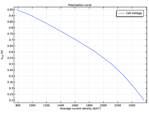
In the associated text field, type Average current density (A/m<sup>2</sup>).
|
|
7
|
|
8
|
In the associated text field, type V<sub>cell</sub> (V).
|
|
1
|
|
2
|
|
4
|
|
5
|
|
6
|
|
1
|
|
2
|
|
3
|
|
4
|
|
5
|
|
6
|
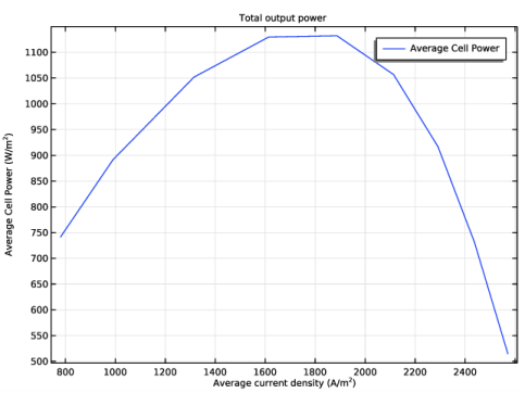
In the associated text field, type Average current density (A/m<sup>2</sup>).
|
|
7
|
|
8
|
In the associated text field, type Average Cell Power (W/m<sup>2</sup>).
|
|
1
|
|
2
|
|
4
|
|
5
|
|
6
|
|
1
|
|
2
|
|
1
|
|
2
|
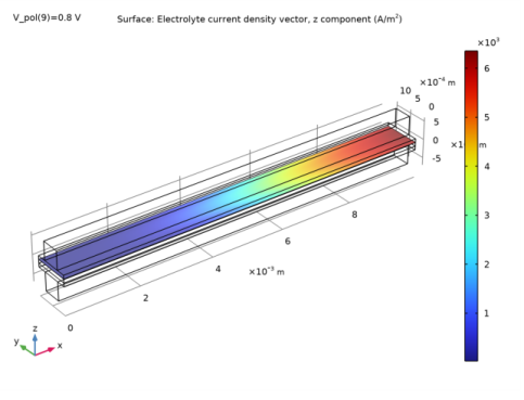
In the Settings window for Surface, click Replace Expression in the upper-right corner of the Expression section. From the menu, choose Component 1 (comp1)>Hydrogen Fuel Cell>Electrolyte current density vector - A/m²>fc.Ilz - Electrolyte current density vector, z component.
|
|
1
|
|
3
|
|
4
|