PDF

Steam Reformer
Introduction
In fuel cell power generators, a steam reformer unit typically produces the hydrogen needed for the fuel cell stack. This example illustrates the modeling of such a steam reformer. The tightly coupled system of mass, energy, and momentum equations used to describe the steam reformer is readily set up using the predefined physics interfaces of the Chemical Reaction Engineering Module.
Depending on the downstream fuel cell type, the carbon monoxide that forms through the reverse water-gas shift (WGS) reaction may poison the fuel cell catalyst. Therefore, after setting up the model, changes are made to the setup to investigate how to decrease the amount of carbon monoxide formed. Three different setups are modeled:
Model Definition
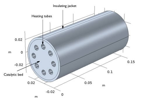
Figure 1 shows the geometry of the reformer. The reformation chemistry occurs in a porous catalytic bed where energy is supplied through heating tubes to drive the endothermic process. The reactor is enclosed in an insulating jacket.
Figure 1: Geometry of the steam reformer unit.
In this example, propane and steam enters the reactor with a steam-to-carbon ratio of 3 mol H2O per mol C. Operating with steam-to-carbon ratios between 2.5 and 4.5 mol/mol is common practice in industry to suppress carbon formation reactions (Ref. 2). Carbon formation is not included in this model, but an example of how to model this can be found in the model Carbon Deposition in Heterogeneous Catalysis, in the Application Library of the Chemical Reaction Engineering Module.
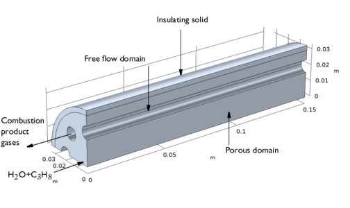
For heating purposes, hot gases from a burner are passed through a number of tubes perforating the reactor bed. The modeled domain can be reduced due to symmetry, see Figure 2.
Figure 2: Making use of symmetry, the modeling domain is reduced to a quarter of the full geometry.
In the reformer, water and propane react to form hydrogen and carbon dioxide:
(1)
An overall kinetic model has been established from experiments (Ref. 1), where the reaction rate (SI unit: mol/(m3·s)) has been found to be first order in the propane concentration:
The rate constant follows Arrhenius equation, with the temperature dependence:
where the frequency factor A is 7·105 s-1 and the activation energy Ea is 83.14 kJ/mol.
In the presence of hydrogen and carbon dioxide there is a probability to produce carbon monoxide through the reverse water gas shift reaction:
(2)
In this model, the reaction rate expression is described by the mass action law
(3)
where kf and kr are the forward and reverse rate constants, respectively. The forward rate constant is set up with an Arrhenius expression, while the reverse rate constant is defined using the concentration equilibrium constant Kc
The water-gas shift reaction is mildly exothermic in its forward direction and the contribution from the reverse direction thus increases with temperature. Production of carbon monoxide is undesirable since hydrogen levels decrease, and carbon monoxide acts as a poison for the catalyst in the downstream fuel cell. Even low levels of carbon monoxide could be harmful for the downstream catalyst, and it is therefore important to include this reaction in the model.
Fluid Flow — reformer Bed
The flow of gaseous species through the reformer bed is described by Darcy’s law:
Here, ρ denotes the gas density (SI unit: kg/m3), η the viscosity (SI unit: Pa·s), κ the permeability of the porous medium (SI unit: m2), and psr is the pressure in the reformer bed (SI unit: Pa). The Darcy’s law equation is, in this example, solved with the Darcy’s law interface.
The inlet and outlet boundary conditions describe a 50 Pa pressure drop across the bed. All other boundaries are impervious, corresponding to the condition:
Energy Transport — reformer Bed
A one-equation approach is used to describe the average temperature distribution in the porous bed:
The effective thermal conductivity of the bed, keff (SI unit: W/(m·K)), is given by:
In the above equations, the indices “f” and “pm” denote fluid and porous matrix, respectively, and ε is the volume fraction of the fluid phase. The effective volumetric heat capacity of the bed is given by:
Furthermore, Tsr (SI unit: K) is the temperature in the bed, Q (SI unit: W/m3) represents a heat source, and u (SI unit: m/s) the fluid velocity. The equation is modeled using the Heat Transfer in Porous Media interface.
Assuming that the porous medium is homogeneous and isotropic, the steady-state equation becomes
(4)
The heat source Q (SI unit: J/(m3·s) due to reaction is
,
where Hj (SI unit: J/(mol·K)) is the enthalpy of reaction for reaction j, and rj is the reaction rate. Steam reformation of propane is endothermic, with an enthalpy of reaction of H = 410 kJ/mol. The two enthalpy of reaction are derived automatically from Thermodynamics.
Equation 4 also accounts for the conductive heat transfer in the insulating jacket. As no reactions occur in this domain, the description reduces to:
where ki is the thermal conductivity (W/(m·K)) of the insulating material.
The temperature of the gas is 700 K at the inlet. At the outlet, it is assumed that convective heat transport is dominant:
The heat exchange between the bed and the tubes is described by:
(5)
where hht is the heat transfer coefficient (SI unit: W/(m2·K)) and T (SI unit: K) is the temperature of the heating tubes. A similar expression describes the heat flux from the insulating jacket to the surroundings:
where hj is the heat transfer coefficient of the jacket (SI unit: W/(m2·K)) and Tamb (SI unit: K) is the ambient temperature.
Mass Transport — reformer Bed
The Transport of Concentrated Species interface gives the equations for the mass transport. The mass-balance equations for the model are the Maxwell-Stefan diffusion and convection equations at steady state:
In the equations above, ρ denotes the density (SI unit: kg/m3), ωi is the mass fraction of species i, xk is the molar fraction of species k, is the ik component of the effective multicomponent Fick diffusivity (SI unit: m2/s). denotes the effective generalized thermal diffusion coefficient (SI unit: kg/(m·s)), T (SI unit: K) is the temperature, and Ri (SI unit: kg/(m3·s)) the reaction rate. The mass-balances are set up and solved with the Transport of Concentrated Species interface. The effective parameters accounts for the impact of porosity on the diffusivity, this model uses the Millington and Quirk model:
The inlet weight fraction of propane is 0.28. At the outlet, the convective flux condition is used:
All other boundaries use the insulating or symmetry condition.
Fluid Flow — heating Tubes
The flow of heating gas in the tubes is described by the weakly compressible Navier-Stokes equations at steady-state:
where ρ (SI unit: kg/m3) denotes density, u (SI unit: m/s) represents the velocity, μ (SI unit: kg/(m· s)) denotes dynamic viscosity, and p (SI unit: Pa) equals the pressure in the tubes.
The boundary conditions for the walls and outlet are
At the outlet, viscous stresses are ignored and the pressure is set to the reference pressure. For the inlet boundary condition, fully developed flow is assumed and solved for using an average velocity.
The Laminar Flow interface sets up and solves the Navier-Stokes equations and is here used to model the gas flow in the tubes. Since the flow is nonisothermal, the Heat Transfer in Fluids interface is also used. These interfaces are coupled through the Nonisothermal Flow multiphysics coupling feature.
Energy Transport — heating Tubes
The energy transport in heating tubes is described by:
where kht is the thermal conductivity (SI unit: W/(m·K)) of the heating gas. The temperature of the gas is 900 K at the inlet. Also this energy transport is modeled with the Heat Transfer in Fluids interface.
At the outlet, it is assumed that convective heat transport is dominant:
The heat exchange between the bed and tubes is given by:
This is the same heat flux as given by Equation 5, but with reversed sign.
Results and Discussion
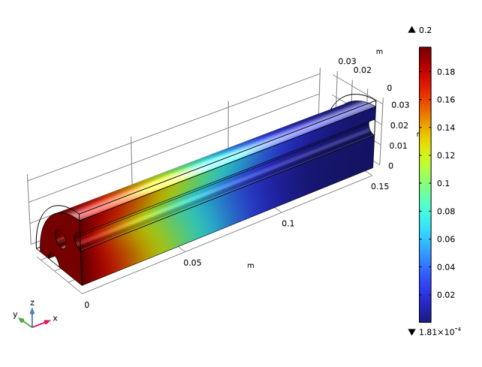
Figure 3 shows the mass fraction of propane in the reformer bed in the countercurrent setup. The inlet mass fraction is 0.20 while the fraction at the outlet is close to zero.
Figure 3: Mass fraction distribution of propane in the reformer bed. Counter current setup.
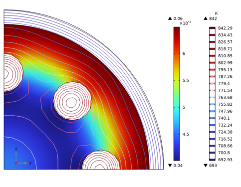
Figure 4, a cut plane plot of the countercurrent dataset, shows the mass fraction of propane in the bed, half way down the reactor length. The temperature in the cut plane is illustrated with contour lines. The mass fraction distribution in the cut plane is small and the heat supplied by the tubes is thus sufficient to make use of the entire catalytic volume. Figure 4 confirms the picture in the previous surface plot, namely that about 75% of the propane has been reformed already half way through the reactor.
Figure 4: Mass fraction distribution of propane in a cut plane half way down the reactor length. Countercurrent setup.
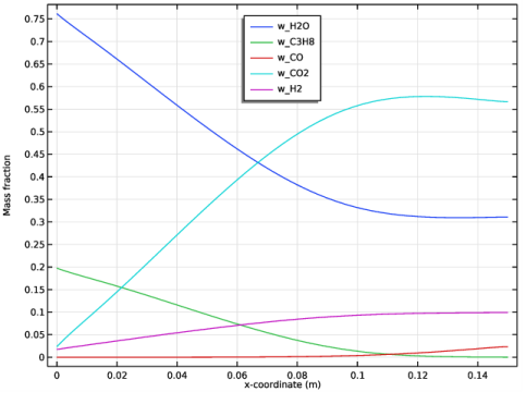
Figure 5 shows the mass fractions of all reacting species in the bed, evaluated along the reactor centerline. CO is formed as a result of the reverse water-gas shift reaction and at
Figure 5: Mass fraction of reacting species as function of bed length, plotted along the reactor centerline. Countercurrent setup.
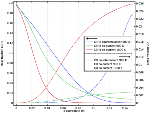
the exit of the bed the mass fraction of CO is a few percent. Depending on the downstream catalyst this may pose a problem. Therefore, two additional reformer setups are modeled to investigate how to decrease the amount of CO formed. The propane and carbon monoxide levels along the bed centerline for all three setups are shown in Figure 7. It is evident that a cocurrent setup, keeping the same inlet temperature for the heating media (900 K), decreases the amount of CO formed in the bed. This effect is mainly due to the lower conversion of propane, resulting in less carbon dioxide, but also an effect of the different temperature profiles in the compared setups. Increasing the heating media temperature to 1000 K in the cocurrent case increases the conversion of propane in the bed, and as a result, the amount of CO formed. Still, with this setup (cocurrent 1000 K) it is possible to decrease the reactor length to 0.1 m while keeping the same level of conversion of propane but not increasing the amount of CO formed.
Figure 6: Mass fraction for propane and carbon monoxide along the bed centerline. Three different setups are shown (countercurrent 900 K, cocurrent 900 K, and cocurrent 1000 K).
.
Figure 7: Reactor temperature as a function of position, plotted along the reactor centerline (solid lines) as well as along one of the tube walls (dashed lines).
Figure 7 shows the temperature along the centerline of the bed, as well as the temperature along one of the tube walls. The gas of the heating tubes enters at 900 K or 1000 K, depending on the setup, and exits at approximately 716 K, 740 K, and 810 K for the cases countercurrent, cocurrent 900 K, and cocurrent 1000 K, respectively. The gas temperature in the reformer bed is 700 K at the inlet for all three setups. For the countercurrent case, the temperature goes through a minimum (due to the endothermic steam reforming reaction), after which it increases and finally exits with an average temperature of 860 K (not shown in the plot). The average exit temperatures (not shown in plot) for the cocurrent cases are both lower than for the countercurrent case, which is beneficial for the forward water-gas shift reaction (decreases CO formation).
Figure 8: Temperature distributions in the reformer system, including the reformer bed and insulating wall (slices), and heating tubes (surface). Arrows indicate total heat flux on part of the symmetry surface for the bed and heating tubes. (a) Countercurrent setup, (b) Cocurrent 1000 K setup.
The energy exchange between the heating tubes and reformer bed is clearly illustrated in Figure 8, showing both the countercurrent and the cocurrent setup (1000 K).
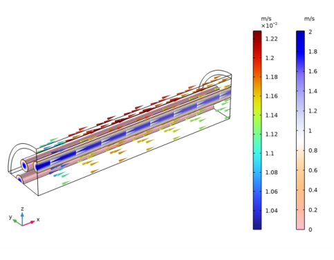
Figure 9 shows, for the cocurrent 1000 K setup, the velocity fields of both the heating gas in the tubes and the reacting gas in the bed. The flow in the heating tubes is laminar and the parabolic velocity distribution is clearly seen. The gas velocity in the porous bed is relatively stable throughout the reactor. This is not the case for the countercurrent setup where the gas velocity in the bed increases much faster along the bed (not shown) due to the temperature increase down the reactor.
Figure 9: Velocity fields of the heating tubes and the reformer bed. Cocurrent 1000 K setup.
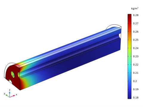
Figure 10 illustrates, for the cocurrent 1000 K setup, the associated density variations in the reformer bed, accounting for both composition and temperature effects. The density variations are all present close to the bed inlet. As for the velocity, the density plot for the countercurrent case is quite different, with a steady decrease in density along the bed length (not shown).
Figure 10: Overall gas density in the reformer bed. Cocurrent 1000 K setup.
In summary, this example illustrates the simulation of a reactor described by fully coupled mass, energy, and flow equations.
Reference
1. P.Gateau, Design of Reactors and Heat Exchange Systems to Optimize a Fuel Cell Reformer, Proceedings of the COMSOL User’s Conference Grenoble, 2007.
2. Moulijn, Jacob A., Makkee, Michiel, van Diepen, Annelies E., Chemical Process Technology, 1st edition, John Wiley & Sons, 2001.
Application Library path: Chemical_Reaction_Engineering_Module/Reactors_with_Porous_Catalysts/steam_reformer
Modeling Instructions
From the File menu, choose New.
New
In the New window, click  Blank Model.
Begin by adding a Thermodynamic system including all the chemical species present in the system.
Global Definitions
In the Physics toolbar, click  Thermodynamics and choose Thermodynamic System.
Select System
1
Go to the Select System window.
2
Click Next in the window toolbar.
Select Species
1
Go to the Select Species window.
2
In the Species list, select propane (74-98-6, C3H8).
3
Click  Add Selected.
4
In the Species list, select water (7732-18-5, H2O).
5
Click  Add Selected.
6
In the Species list, select hydrogen (1333-74-0, H2).
7
Click  Add Selected.
8
In the Species list, select carbon dioxide (124-38-9, CO2).
9
Click  Add Selected.
10
In the Species list, select carbon monoxide (630-08-0, CO).
11
Click  Add Selected.
12
Click Next in the window toolbar.
Select Thermodynamic Model
1
Go to the Select Thermodynamic Model window.
2
Click Finish in the window toolbar.
Global Definitions
Gas System 1 (pp1)
With a Thermodynamic system in place, it is straightforward to set up the Chemistry interface using Generate Chemistry.
1
In the Model Builder window, under Global Definitions>Thermodynamics right-click Gas System 1 (pp1) and choose Generate Chemistry.
Select Species
1
Go to the Select Species window.
2
Click  Add All.
3
Click Next in the window toolbar.
Chemistry Settings
1
Go to the Chemistry Settings window.
2
From the Mass transfer list, choose Concentrated species.
3
Click Finish in the window toolbar.
Global Definitions
A set of parameters that are useful when building the model are available in a text file. In the next steps load these into the parameters section.
Parameters 1
1
In the Model Builder window, under Global Definitions click Parameters 1.
2
In the Settings window for Parameters, locate the Parameters section.
3
Click  Load from File.
4
Geometry 1
Now create the geometry. To simplify this step, insert a prepared geometry sequence:
1
In the Model Builder window, under Component 1 (comp1) click Geometry 1.
2
In the Geometry toolbar, point to Import/Export and choose Insert Sequence.
3
4
Click Build All in the Geometry toolbar.
Now create explicit selections for the domains and boundaries in the geometry. Selections facilitate the work of assigning materials, setting boundary conditions, and plot the results.
Definitions
Catalytic Bed
1
In the Definitions toolbar, click  Explicit.
2
In the Settings window for Explicit, type Catalytic Bed in the Label text field.
3
Remaining explicit definitions
Analogous to the explicit definition for the Catalytic Bed, proceed to create the following explicit definitions:
Also create a union selection containing all inlet and outlet boundaries. This will be used to refine the mesh in these areas.
Inlets and Outlets
1
In the Definitions toolbar, click  Union.
2
In the Settings window for Union, type Inlets and Outlets in the Label text field.
3
Locate the Geometric Entity Level section. From the Level list, choose Boundary.
4
Locate the Input Entities section. Under Selections to add, click  Add.
5
In the Add dialog box, in the Selections to add list, choose Bed Inlet, Bed Outlet, Tubes Inlet, and Tubes Outlet.
6
Integration 1 (intop1)
1
In the Definitions toolbar, click  Nonlocal Couplings and choose Integration.
2
In the Settings window for Integration, locate the Source Selection section.
3
From the Geometric entity level list, choose Boundary.
4
Create the materials for hot gas (air), insulating jacket, and catalytic bed.
Materials
Catalyst
1
In the Model Builder window, under Component 1 (comp1) right-click Materials and choose Blank Material.
2
In the Settings window for Material, type Catalyst in the Label text field.
Insulation
1
Right-click Materials and choose Blank Material.
2
In the Settings window for Material, type Insulation in the Label text field.
3
Locate the Geometric Entity Selection section. From the Selection list, choose Jacket.
Add Material
1
In the Home toolbar, click  Add Material to open the Add Material window.
2
Go to the Add Material window.
3
4
Click Add to Component in the window toolbar.
Materials
Air (mat3)
1
In the Settings window for Material, locate the Geometric Entity Selection section.
2
From the Selection list, choose Heating Tubes.
Porous Material 1 (pmat1)
1
Right-click Materials and choose More Materials>Porous Material.
2
In the Settings window for Porous Material, locate the Geometric Entity Selection section.
3
From the Selection list, choose Catalytic Bed.
Now add the physics interfaces. When they are all added, go back to each of the interfaces, assign them to their domains, and add the necessary feature nodes. Based on this, COMSOL automatically detects which material properties are needed and you can then fill them in.
Add Physics
1
In the Home toolbar, click  Add Physics to open the Add Physics window.
2
Go to the Add Physics window.
3
In the tree, select Chemical Species Transport>Transport of Concentrated Species (tcs).
4
Click Add to Component 1 in the window toolbar.
Transport of Concentrated Species (tcs)
1
In the Settings window for Transport of Concentrated Species, locate the Transport Mechanisms section.
2
Select the Mass transfer in porous media check box.
3
Click to expand the Dependent Variables section. In the Number of species text field, type 5.
4
In the Mass fractions table, enter the following settings:
Add Physics
1
Go to the Add Physics window.
2
In the tree, select Fluid Flow>Porous Media and Subsurface Flow>Darcy’s Law (dl).
3
Click Add to Component 1 in the window toolbar.
Darcy’s Law (dl)
1
In the Settings window for Darcy’s Law, locate the Physical Model section.
2
In the pref text field, type p_ref.
3
Click to expand the Dependent Variables section. In the Pressure text field, type p_sr.
Add Physics
1
Go to the Add Physics window.
2
In the tree, select Heat Transfer>Porous Media>Heat Transfer in Porous Media (ht).
3
Click Add to Component 1 in the window toolbar.
Heat Transfer in Porous Media (ht)
1
In the Settings window for Heat Transfer in Porous Media, click to expand the Dependent Variables section.
2
In the Temperature text field, type T_sr.
Add Physics
1
Go to the Add Physics window.
2
In the tree, select Fluid Flow>Nonisothermal Flow>Laminar Flow.
3
Click Add to Component 1 in the window toolbar.
4
In the Home toolbar, click  Add Physics to close the Add Physics window.
Laminar Flow (spf)
1
In the Settings window for Laminar Flow, locate the Physical Model section.
2
In the pref text field, type p_ref.
3
Click to expand the Dependent Variables section. In the Pressure text field, type p_tubes.
Heat Transfer in Fluids 2 (ht2)
1
In the Model Builder window, under Component 1 (comp1) click Heat Transfer in Fluids 2 (ht2).
2
In the Settings window for Heat Transfer in Fluids, click to expand the Dependent Variables section.
3
In the Temperature text field, type T_tubes.
Chemistry (chem)
1
In the Model Builder window, under Component 1 (comp1) click Chemistry (chem).
2
In the Settings window for Chemistry, locate the Species Matching section.
3
From the Species solved for list, choose Transport of Concentrated Species.
4
Find the Bulk species subsection. In the table, enter the following settings:
Reaction 1
1
In the Physics toolbar, click  Domains and choose Reaction.
2
In the Settings window for Reaction, locate the Reaction Formula section.
3
In the Formula text field, type C3H8 + H2O => H2 + CO2.
4
Click Balance in the upper-right corner of the Reaction Formula section.
5
Locate the Reaction Rate section. From the list, choose User defined.
6
In the rj text field, type chem.kf_1*chem.c_C3H8.
7
Find the Volumetric overall reaction order subsection. In the Forward text field, type 1.
8
Locate the Rate Constants section. Select the Use Arrhenius expressions check box.
9
In the Af text field, type A.
10
In the Ef text field, type Ea.
Reaction 2
1
In the Physics toolbar, click  Domains and choose Reaction.
2
In the Settings window for Reaction, locate the Reaction Formula section.
3
In the Formula text field, type CO+H2O<=>CO2+H2.
4
Click Apply.
5
Locate the Rate Constants section. Select the Specify equilibrium constant check box.
6
Select the Use Arrhenius expressions check box.
7
In the Af text field, type A_wgs.
8
In the Ef text field, type Ea_wgs.
Transport of Concentrated Species in Bed
1
In the Model Builder window, under Component 1 (comp1) click Transport of Concentrated Species (tcs).
2
In the Settings window for Transport of Concentrated Species, type Transport of Concentrated Species in Bed in the Label text field.
3
Locate the Domain Selection section. From the Selection list, choose Catalytic Bed.
4
Locate the Transport Mechanisms section. From the Diffusion model list, choose Maxwell-Stefan.
Initial Values 1
1
In the Model Builder window, under Component 1 (comp1)>Transport of Concentrated Species in Bed (tcs) click Initial Values 1.
2
In the Settings window for Initial Values, locate the Initial Values section.
3
In the ω0,wC3H8 text field, type w_C3H8_in.
4
In the ω0,wH2 text field, type w_H2_in.
5
In the ω0,wCO2 text field, type w_CO2_in.
6
In the ω0,wCO text field, type w_CO_in.
Porous Medium 1
1
In the Physics toolbar, click  Domains and choose Porous Medium.
2
In the Settings window for Porous Medium, locate the Domain Selection section.
3
From the Selection list, choose Catalytic Bed.
Fluid 1
1
In the Model Builder window, click Fluid 1.
2
In the Settings window for Fluid, locate the Density section.
3
From the MwH2O list, choose Molar mass (chem/H2O).
4
From the MwC3H8 list, choose Molar mass (chem/C3H8).
5
From the MwH2 list, choose Molar mass (chem/H2).
6
From the MwCO2 list, choose Molar mass (chem/CO2).
7
From the MwCO list, choose Molar mass (chem/CO).
8
Locate the Convection section. From the u list, choose Darcy’s velocity field (dl/porous1).
9
Locate the Diffusion section. In the table, enter the following settings:
Porous Matrix 1
1
In the Model Builder window, click Porous Matrix 1.
2
In the Settings window for Porous Matrix, locate the Matrix Properties section.
3
From the εp list, choose From material.
Reaction Sources 1
1
In the Physics toolbar, click  Domains and choose Reaction Sources.
2
In the Settings window for Reaction Sources, locate the Domain Selection section.
3
From the Selection list, choose Catalytic Bed.
4
Locate the Reactions section. From the RwC3H8 list, choose Reaction rate for species C3H8 (chem).
5
From the RwH2 list, choose Reaction rate for species H2 (chem).
6
From the RwCO2 list, choose Reaction rate for species CO2 (chem).
7
From the RwCO list, choose Reaction rate for species CO (chem).
8
Locate the Reacting Volume section. From the Reacting volume list, choose Pore volume.
Inflow 1
In the Physics toolbar, click  Boundaries and choose Inflow.
Definitions
Variables 1
1
In the Home toolbar, click  Variables and choose Local Variables.
2
In the Settings window for Variables, locate the Variables section.
3
Transport of Concentrated Species in Bed (tcs)
Inflow 1
1
In the Model Builder window, under Component 1 (comp1)>Transport of Concentrated Species in Bed (tcs) click Inflow 1.
2
In the Settings window for Inflow, locate the Boundary Selection section.
3
From the Selection list, choose Bed Inlet.
4
Locate the Inflow section. From the Mixture specification list, choose Mass flow rates.
5
In the Jin,wC3H8 text field, type J_in_C3H8.
6
In the Jin,wH2 text field, type J_in_H2.
7
In the Jin,wCO2 text field, type J_in_CO2.
8
In the Jin,wCO text field, type J_in_CO.
Outflow 1
1
In the Physics toolbar, click  Boundaries and choose Outflow.
2
In the Settings window for Outflow, locate the Boundary Selection section.
3
From the Selection list, choose Bed Outlet.
Darcy’s Law in Bed
1
In the Model Builder window, under Component 1 (comp1) click Darcy’s Law (dl).
2
In the Settings window for Darcy’s Law, type Darcy's Law in Bed in the Label text field.
3
Locate the Domain Selection section. From the Selection list, choose Catalytic Bed.
Fluid 1
1
In the Model Builder window, under Component 1 (comp1)>Darcy’s Law in Bed (dl)>Porous Medium 1 click Fluid 1.
2
In the Settings window for Fluid, locate the Fluid Properties section.
3
From the ρ list, choose Density (tcs).
4
From the μ list, choose Dynamic viscosity (chem).
Inlet 1
1
In the Physics toolbar, click  Boundaries and choose Inlet.
2
In the Settings window for Inlet, locate the Boundary Condition section.
3
4
Locate the Pressure section. In the p0 text field, type p_in_sr.
5
Locate the Boundary Selection section. From the Selection list, choose Bed Inlet.
Outlet 1
1
In the Physics toolbar, click  Boundaries and choose Outlet.
2
In the Settings window for Outlet, locate the Boundary Selection section.
3
From the Selection list, choose Bed Outlet.
4
Locate the Boundary Condition section. From the list, choose Pressure.
Symmetry 1
1
In the Physics toolbar, click  Boundaries and choose Symmetry.
2
In the Settings window for Symmetry, locate the Boundary Selection section.
3
From the Selection list, choose Bed Symmetry.
Heat Transfer in Porous Media in Bed
1
In the Model Builder window, under Component 1 (comp1) click Heat Transfer in Porous Media (ht).
2
In the Settings window for Heat Transfer in Porous Media, type Heat Transfer in Porous Media in Bed in the Label text field.
3
Fluid 1
1
In the Model Builder window, under Component 1 (comp1)>Heat Transfer in Porous Media in Bed (ht)>Porous Medium 1 click Fluid 1.
2
In the Settings window for Fluid, locate the Heat Convection section.
3
From the u list, choose Darcy’s velocity field (dl/porous1).
4
Locate the Heat Conduction, Fluid section. From the kf list, choose Thermal conductivity (chem).
5
Locate the Thermodynamics, Fluid section. From the ρf list, choose Density (tcs).
6
From the Cp,f list, choose Heat capacity at constant pressure (chem).
7
From the γ list, choose Ratio of specific heats (chem).
Porous Matrix 1
1
In the Model Builder window, click Porous Matrix 1.
2
In the Settings window for Porous Matrix, locate the Matrix Properties section.
3
From the Define list, choose Solid phase properties.
Initial Values 1
1
In the Model Builder window, under Component 1 (comp1)>Heat Transfer in Porous Media in Bed (ht) click Initial Values 1.
2
In the Settings window for Initial Values, locate the Initial Values section.
3
In the Tsr text field, type T_in_sr.
Solid 1
1
In the Physics toolbar, click  Domains and choose Solid.
2
In the Settings window for Solid, locate the Domain Selection section.
3
From the Selection list, choose Jacket.
Temperature 1
1
In the Physics toolbar, click  Boundaries and choose Temperature.
2
In the Settings window for Temperature, locate the Boundary Selection section.
3
From the Selection list, choose Bed Inlet.
4
Locate the Temperature section. In the T0 text field, type T_in_sr.
Outflow 1
1
In the Physics toolbar, click  Boundaries and choose Outflow.
2
In the Settings window for Outflow, locate the Boundary Selection section.
3
From the Selection list, choose Bed Outlet.
Heat Flux 1
1
In the Physics toolbar, click  Boundaries and choose Heat Flux.
2
In the Settings window for Heat Flux, locate the Boundary Selection section.
3
From the Selection list, choose Tubes/Bed.
4
Locate the Heat Flux section. From the Flux type list, choose Convective heat flux.
5
In the h text field, type h_tubes.
6
In the Text text field, type T_tubes.
Heat Flux 2
1
In the Physics toolbar, click  Boundaries and choose Heat Flux.
2
In the Settings window for Heat Flux, locate the Boundary Selection section.
3
From the Selection list, choose Jacket/Ambient.
4
Locate the Heat Flux section. From the Flux type list, choose Convective heat flux.
5
In the h text field, type h_j.
6
In the Text text field, type T_amb.
Heat Source 1
1
In the Physics toolbar, click  Domains and choose Heat Source.
2
In the Settings window for Heat Source, locate the Heat Source section.
3
In the Q0 text field, type porosity*chem.Qtot.
4
Locate the Domain Selection section. From the Selection list, choose Catalytic Bed.
Laminar Flow in Heating Tubes
1
In the Model Builder window, under Component 1 (comp1) click Laminar Flow (spf).
2
In the Settings window for Laminar Flow, type Laminar Flow in Heating Tubes in the Label text field.
3
Locate the Domain Selection section. From the Selection list, choose Heating Tubes.
Inlet 1
1
In the Physics toolbar, click  Boundaries and choose Inlet.
2
In the Settings window for Inlet, locate the Boundary Selection section.
3
From the Selection list, choose Tubes Inlet.
4
Locate the Boundary Condition section. From the list, choose Fully developed flow.
5
Locate the Fully Developed Flow section. In the Uav text field, type u_in_tubes.
Outlet 1
1
In the Physics toolbar, click  Boundaries and choose Outlet.
2
In the Settings window for Outlet, locate the Boundary Selection section.
3
From the Selection list, choose Tubes Outlet.
4
Locate the Pressure Conditions section. Select the Normal flow check box.
Symmetry 1
1
In the Physics toolbar, click  Boundaries and choose Symmetry.
2
In the Settings window for Symmetry, locate the Boundary Selection section.
3
From the Selection list, choose Tubes Symmetry.
Heat Transfer in Heating Tubes
1
In the Model Builder window, under Component 1 (comp1) click Heat Transfer in Fluids 2 (ht2).
2
In the Settings window for Heat Transfer in Fluids, type Heat Transfer in Heating Tubes in the Label text field.
3
Locate the Domain Selection section. From the Selection list, choose Heating Tubes.
Initial Values 1
1
In the Model Builder window, under Component 1 (comp1)>Heat Transfer in Heating Tubes (ht2) click Initial Values 1.
2
In the Settings window for Initial Values, locate the Initial Values section.
3
In the Ttubes text field, type T_in_tubes.
Temperature at Inlet
1
In the Physics toolbar, click  Boundaries and choose Temperature.
2
In the Settings window for Temperature, type Temperature at Inlet in the Label text field.
3
Locate the Boundary Selection section. From the Selection list, choose Tubes Inlet.
4
Locate the Temperature section. In the T0 text field, type T_in_tubes.
Outflow 1
1
In the Physics toolbar, click  Boundaries and choose Outflow.
2
In the Settings window for Outflow, locate the Boundary Selection section.
3
From the Selection list, choose Tubes Outlet.
Heat Flux to bed
1
In the Physics toolbar, click  Boundaries and choose Heat Flux.
2
In the Settings window for Heat Flux, type Heat Flux to bed in the Label text field.
3
Locate the Boundary Selection section. From the Selection list, choose Tubes/Bed.
4
Locate the Heat Flux section. From the Flux type list, choose Convective heat flux.
5
In the h text field, type h_tubes.
6
In the Text text field, type T_sr.
Materials
Now, after the physics is set up, you can fill in the required material properties.
Porous Material 1 (pmat1)
1
In the Model Builder window, under Component 1 (comp1)>Materials click Porous Material 1 (pmat1).
2
In the Settings window for Porous Material, locate the Homogenized Properties section.
3
4
Locate the Phase-Specific Properties section. Click  Add Required Phase Nodes.
Solid 1 (pmat1.solid1)
1
In the Model Builder window, click Solid 1 (pmat1.solid1).
2
In the Settings window for Solid, locate the Solid Properties section.
3
From the Material list, choose Catalyst (mat1).
4
In the θs text field, type 1-porosity.
Catalyst (mat1)
1
In the Model Builder window, under Component 1 (comp1)>Materials click Catalyst (mat1).
2
In the Settings window for Material, locate the Material Contents section.
3
Insulation (mat2)
1
In the Model Builder window, click Insulation (mat2).
2
In the Settings window for Material, locate the Material Contents section.
3
Mesh 1
Now add a mesh. The mesh will consist of free quads (bed), free triangles (tube and jacket), boundary layers on the bed/tube boundaries, and boundary layers in the x-direction on the inlets and outlets selection.
Free Quad 1
1
In the Mesh toolbar, click  Boundary and choose Free Quad.
2
In the Settings window for Free Quad, locate the Boundary Selection section.
3
From the Selection list, choose Bed Inlet.
Size 1
1
In the Mesh toolbar, click Size Attribute and choose Normal.
2
In the Settings window for Size, locate the Element Size section.
3
Click the Custom button.
4
Locate the Element Size Parameters section. Select the Maximum element size check box.
5
Size
1
In the Model Builder window, under Component 1 (comp1)>Mesh 1 click Size.
2
In the Settings window for Size, locate the Element Size section.
3
Click the Custom button.
4
Locate the Element Size Parameters section. In the Maximum element size text field, type 2e-3.
5
In the Minimum element size text field, type 1e-3.
Free Triangular 1
1
In the Mesh toolbar, click  Boundary and choose Free Triangular.
2
In the Settings window for Free Triangular, locate the Boundary Selection section.
3
From the Selection list, choose Tubes Outlet.
4
Boundary Layers 1
1
In the Mesh toolbar, click  Boundary Layers.
2
In the Settings window for Boundary Layers, locate the Geometric Entity Selection section.
3
From the Geometric entity level list, choose Boundary.
4
From the Selection list, choose Tubes Outlet.
5
Boundary Layer Properties
1
In the Model Builder window, click Boundary Layer Properties.
2
In the Settings window for Boundary Layer Properties, locate the Edge Selection section.
3
Click  Paste Selection.
4
In the Paste Selection dialog box, type 5 8 16 17 19 21 24 27 in the Selection text field.
5
Click OK. Alternatively, click in the Graphics window to select the bed/tube boundaries.
6
In the Settings window for Boundary Layer Properties, locate the Layers section.
7
In the Number of layers text field, type 3.
8
From the Thickness specification list, choose First layer.
9
In the Thickness text field, type 3e-4.
Swept 1
In the Mesh toolbar, click  Swept.
Distribution 1
1
In the Mesh toolbar, click  Distribution.
2
In the Settings window for Distribution, locate the Distribution section.
3
In the Number of elements text field, type 50.
4
Click  Build All.
Boundary Layers 2
1
In the Mesh toolbar, click  Boundary Layers.
2
In the Settings window for Boundary Layers, click to expand the Transition section.
3
Clear the Smooth transition to interior mesh check box.
Boundary Layer Properties
1
In the Model Builder window, click Boundary Layer Properties.
2
In the Settings window for Boundary Layer Properties, locate the Geometric Entity Selection section.
3
From the Selection list, choose Inlets and Outlets.
4
Locate the Layers section. From the Thickness specification list, choose First layer.
5
In the Number of layers text field, type 6.
6
In the Thickness text field, type 0.0003.
7
Click  Build All.
Use the Statistics feature to get information about the mesh.
8
In the Model Builder window, right-click Mesh 1 and choose Statistics.
Add Study
1
In the Home toolbar, click  Add Study to open the Add Study window.
2
Go to the Add Study window.
3
Find the Studies subsection. In the Select Study tree, select General Studies>Stationary.
4
5
In the Home toolbar, click  Add Study to close the Add Study window.
Study 1
Solution 1 (sol1)
In the Study toolbar, click  Show Default Solver.
Step 1: Stationary
1
In the Settings window for Stationary, locate the Physics and Variables Selection section.
2
In the table, clear the Solve for check boxes for Chemistry (chem), Transport of Concentrated Species in Bed (tcs), Heat Transfer in Porous Media in Bed (ht), Laminar Flow in Heating Tubes (spf), and Heat Transfer in Heating Tubes (ht2).
3
In the table, clear the Solve for check box for Nonisothermal Flow 1 (nitf1).
Step 2: Stationary 1
1
Right-click Study 1>Step 1: Stationary and choose Duplicate.
2
In the Settings window for Stationary, locate the Physics and Variables Selection section.
3
Step 3: Stationary 2
1
Right-click Step 2: Stationary 1 and choose Duplicate.
2
In the Settings window for Stationary, locate the Physics and Variables Selection section.
3
In the table, select the Solve for check boxes for Chemistry (chem), Transport of Concentrated Species in Bed (tcs), Darcy’s Law in Bed (dl), Heat Transfer in Porous Media in Bed (ht), and Heat Transfer in Heating Tubes (ht2).
4
In the table, select the Solve for check box for Nonisothermal Flow 1 (nitf1).
Solution 1 (sol1)
1
In the Study toolbar, click  Show Default Solver.
2
In the Model Builder window, expand the Solution 1 (sol1) node.
3
In the Model Builder window, expand the Study 1>Solver Configurations>Solution 1 (sol1)>Stationary Solver 3 node.
4
Right-click Study 1>Solver Configurations>Solution 1 (sol1)>Stationary Solver 3 and choose Fully Coupled.
5
In the Study toolbar, click  Compute.
Results
In the first part of the results processing, modify two of the default plots to get Figure 3 and Figure 4.
Concentration, C3H8, Surface (tcs)
1
In the Model Builder window, under Results click Concentration, C3H8, Surface (tcs).
2
In the Settings window for 3D Plot Group, click to expand the Title section.
3
From the Title type list, choose None.
4
Locate the Color Legend section. Select the Show maximum and minimum values check box.
Surface 1
1
In the Model Builder window, expand the Concentration, C3H8, Surface (tcs) node, then click Surface 1.
2
In the Settings window for Surface, locate the Expression section.
3
In the Expression text field, type w_C3H8.
4
In the Concentration, C3H8, Surface (tcs) toolbar, click  Plot.
5
Click the  Zoom Extents button in the Graphics toolbar.
Mass fraction, C3H8, Surface (tcs)
1
In the Model Builder window, under Results click Concentration, C3H8, Surface (tcs).
2
In the Settings window for 3D Plot Group, type Mass fraction, C3H8, Surface (tcs) in the Label text field.
This is Figure 3. Continue by setting up Figure 4, that is plotting the mass fraction of propane, and the bed temperature, half way down the reactor length. This will illustrate how well the catalyst in the bed is utilized. Begin by creating a cut plane dataset.
Cut Plane 1
1
In the Results toolbar, click  Cut Plane.
2
In the Settings window for Cut Plane, locate the Plane Data section.
3
In the x-coordinate text field, type L/2.
4
w_C3H8 and T at L/2
1
In the Results toolbar, click  3D Plot Group.
2
In the Settings window for 3D Plot Group, type w_C3H8 and T at L/2 in the Label text field.
3
Locate the Data section. From the Dataset list, choose Cut Plane 1.
4
Locate the Title section. From the Title type list, choose None.
5
Locate the Color Legend section. Select the Show maximum and minimum values check box.
6
Select the Show units check box.
Surface 1
1
Right-click w_C3H8 and T at L/2 and choose Surface.
2
In the Settings window for Surface, locate the Expression section.
3
In the Expression text field, type w_C3H8.
Contour 1
1
In the Model Builder window, right-click w_C3H8 and T at L/2 and choose Contour.
2
In the Settings window for Contour, locate the Expression section.
3
In the Expression text field, type chem.T.
4
In the w_C3H8 and T at L/2 toolbar, click  Plot.
5
Locate the Coloring and Style section. From the Color table list, choose Wave.
6
Click the  Go to YZ View button in the Graphics toolbar.
7
Click the  Show Grid button in the Graphics toolbar.
8
Click the  Zoom Extents button in the Graphics toolbar.
This is Figure 4. Now, plot the mass fractions for all chemical species along the center line of the reactor bed. This is achieved by setting up a 1D Plot Group with one Line Graph for each chemical species. The resulting plot is Figure 5.
9
Click the  Go to Default View button in the Graphics toolbar.
Counter current mass fractions
1
In the Home toolbar, click  Add Plot Group and choose 1D Plot Group.
2
In the Settings window for 1D Plot Group, type Counter current mass fractions in the Label text field.
3
Click to expand the Title section. From the Title type list, choose None.
Line Graph 1
1
Right-click Counter current mass fractions and choose Line Graph.
2
3
In the Settings window for Line Graph, locate the x-Axis Data section.
4
From the Parameter list, choose Expression.
5
In the Expression text field, type x.
6
Click to expand the Legends section. Select the Show legends check box.
7
Find the Include subsection. Select the Expression check box.
8
Clear the Solution check box.
9
In the Counter current mass fractions toolbar, click  Plot.
Line Graph 2
1
Right-click Line Graph 1 and choose Duplicate.
2
In the Settings window for Line Graph, locate the y-Axis Data section.
3
In the Expression text field, type w_C3H8.
Line Graph 3
1
Right-click Line Graph 2 and choose Duplicate.
2
In the Settings window for Line Graph, locate the y-Axis Data section.
3
In the Expression text field, type w_CO.
Line Graph 4
1
Right-click Line Graph 3 and choose Duplicate.
2
In the Settings window for Line Graph, locate the y-Axis Data section.
3
In the Expression text field, type w_CO2.
Line Graph 5
1
Right-click Line Graph 4 and choose Duplicate.
2
In the Settings window for Line Graph, locate the y-Axis Data section.
3
In the Expression text field, type w_H2.
Counter current mass fractions
1
In the Model Builder window, click Counter current mass fractions.
2
In the Settings window for 1D Plot Group, locate the Plot Settings section.
3
Select the y-axis label check box.
4
5
Locate the Legend section. From the Position list, choose Upper middle.
This is Figure 5.
6
Click the  Zoom Extents button in the Graphics toolbar.
Study 1
From Figure 5 it is evident that some CO is formed. As mentioned in the introduction, in this model a design study is performed to try and minimize the produced CO. The first step in the design study is to change the flow direction in the heating tubes. This is easily done when explicit selections are present. Before continuing, save the current solution and call it "Countercurrent T_in_tubes = 900 K.
Solution 1 (sol1)
In the Model Builder window, under Study 1>Solver Configurations right-click Solution 1 (sol1) and choose Solution>Copy.
Solution 1 - Counter current T_in_tubes = 900 K
1
In the Model Builder window, under Study 1>Solver Configurations click Solution 1 - Copy 1 (sol4).
2
In the Settings window for Solution, type Solution 1 - Counter current T_in_tubes = 900 K in the Label text field.
Laminar Flow in Heating Tubes (spf)
Now, switch to co-current flow by changing the selections for the inlets and outlets of the heating tubes.
Inlet 1
1
In the Model Builder window, under Component 1 (comp1)>Laminar Flow in Heating Tubes (spf) click Inlet 1.
2
In the Settings window for Inlet, locate the Boundary Selection section.
3
From the Selection list, choose Tubes Outlet.
Outlet 1
1
In the Model Builder window, click Outlet 1.
2
In the Settings window for Outlet, locate the Boundary Selection section.
3
From the Selection list, choose Tubes Inlet.
Heat Transfer in Heating Tubes (ht2)
Temperature at Inlet
1
In the Model Builder window, under Component 1 (comp1)>Heat Transfer in Heating Tubes (ht2) click Temperature at Inlet.
2
In the Settings window for Temperature, locate the Boundary Selection section.
3
From the Selection list, choose Tubes Outlet.
Outflow 1
1
In the Model Builder window, click Outflow 1.
2
In the Settings window for Outflow, locate the Boundary Selection section.
3
From the Selection list, choose Tubes Inlet.
Study 1
In the Home toolbar, click  Compute.
Solution 1 (sol1)
In the Model Builder window, under Study 1>Solver Configurations right-click Solution 1 (sol1) and choose Solution>Copy.
Solution 1 - Cocurrent T_in_tubes = 900 K
1
In the Model Builder window, under Study 1>Solver Configurations click Solution 1 - Copy 1 (sol5).
2
In the Settings window for Solution, type Solution 1 - Cocurrent T_in_tubes = 900 K in the Label text field.
Global Definitions
Parameters 1
1
In the Model Builder window, under Global Definitions click Parameters 1.
2
In the Settings window for Parameters, locate the Parameters section.
3
Study 1
In the Home toolbar, click  Compute.
Solution 1 (sol1)
In the Model Builder window, under Study 1>Solver Configurations right-click Solution 1 (sol1) and choose Solution>Copy.
Solution 1 - Cocurrent T_in_tubes = 1000 K
1
In the Model Builder window, under Study 1>Solver Configurations click Solution 1 - Copy 1 (sol6).
2
In the Settings window for Solution, type Solution 1 - Cocurrent T_in_tubes = 1000 K in the Label text field.
Results
Now, plot mass fractions of C3H8 and CO for the three solutions (design cases) in the same plot. Use two y-axes to better visualize the results. When done this will give Figure 6.
w_C3H8 and w_CO along bed midline
1
In the Home toolbar, click  Add Plot Group and choose 1D Plot Group.
2
In the Settings window for 1D Plot Group, type w_C3H8 and w_CO along bed midline in the Label text field.
3
Locate the Title section. From the Title type list, choose None.
C3H8 counter current
1
Right-click w_C3H8 and w_CO along bed midline and choose Line Graph.
2
In the Settings window for Line Graph, type C3H8 counter current in the Label text field.
3
Locate the Data section. From the Dataset list, choose Study 1/Solution 1 - Counter current T_in_tubes = 900 K (sol4).
4
5
Locate the y-Axis Data section. In the Expression text field, type w_C3H8.
6
Locate the x-Axis Data section. From the Parameter list, choose Expression.
7
In the Expression text field, type x.
8
Locate the Legends section. Select the Show legends check box.
9
From the Legends list, choose Manual.
10
C3H8 co-current 900 K
1
Right-click C3H8 counter current and choose Duplicate.
2
In the Settings window for Line Graph, type C3H8 co-current 900 K in the Label text field.
3
Locate the Data section. From the Dataset list, choose Study 1/Solution 1 - Cocurrent T_in_tubes = 900 K (sol5).
4
Locate the Legends section. In the table, enter the following settings:
C3H8 co-current 1000 K
1
Right-click C3H8 co-current 900 K and choose Duplicate.
2
In the Settings window for Line Graph, type C3H8 co-current 1000 K in the Label text field.
3
Locate the Data section. From the Dataset list, choose Study 1/Solution 1 - Cocurrent T_in_tubes = 1000 K (sol6).
4
Locate the Legends section. In the table, enter the following settings:
5
In the w_C3H8 and w_CO along bed midline toolbar, click  Plot.
C3H8 co-current 1000 K, C3H8 co-current 900 K, C3H8 counter current
1
In the Model Builder window, under Results>w_C3H8 and w_CO along bed midline, Ctrl-click to select C3H8 counter current, C3H8 co-current 900 K, and C3H8 co-current 1000 K.
2
C3H8 counter current 1
1
In the Settings window for Line Graph, locate the y-Axis Data section.
2
In the Expression text field, type w_CO.
3
Locate the Legends section. In the table, enter the following settings:
4
Click to expand the Coloring and Style section. Find the Line style subsection. From the Line list, choose Dashed.
5
From the Color list, choose Cycle (reset).
C3H8 co-current 900 K 1
1
In the Model Builder window, click C3H8 co-current 900 K 1.
2
In the Settings window for Line Graph, locate the Coloring and Style section.
3
Find the Line style subsection. From the Line list, choose Dashed.
4
Locate the Legends section. In the table, enter the following settings:
5
Locate the y-Axis Data section. In the Expression text field, type w_CO.
CO co-current 1000 K
1
In the Model Builder window, click C3H8 co-current 1000 K 1.
2
In the Settings window for Line Graph, locate the y-Axis Data section.
3
In the Expression text field, type w_CO.
4
Locate the Coloring and Style section. Find the Line style subsection. From the Line list, choose Dashed.
5
Locate the Legends section. In the table, enter the following settings:
6
In the Label text field, type CO co-current 1000 K.
CO co-current 900 K
1
In the Model Builder window, under Results>w_C3H8 and w_CO along bed midline click C3H8 co-current 900 K 1.
2
In the Settings window for Line Graph, type CO co-current 900 K in the Label text field.
CO counter current 900 K
1
In the Model Builder window, under Results>w_C3H8 and w_CO along bed midline click C3H8 counter current 1.
2
In the Settings window for Line Graph, type CO counter current 900 K in the Label text field.
w_C3H8 and w_CO along bed midline
1
In the Model Builder window, click w_C3H8 and w_CO along bed midline.
2
In the Settings window for 1D Plot Group, locate the Plot Settings section.
3
Select the x-axis label check box.
4
Select the y-axis label check box.
5
6
Select the Two y-axes check box.
7
Select the Secondary y-axis label check box.
8
9
In the table, select the Plot on secondary y-axis check boxes for CO counter current 900 K, CO co-current 900 K, and CO co-current 1000 K.
10
In the w_C3H8 and w_CO along bed midline toolbar, click  Plot.
11
Locate the Legend section. From the Position list, choose Middle right.
12
In the w_C3H8 and w_CO along bed midline toolbar, click  Plot.
13
Click the  Zoom Extents button in the Graphics toolbar.
This is Figure 6.
Now plot the temperature profiles along the bed centerline and along the side of one of the heating tubes. Utilize the plot group just created by duplicating it and modify the expressions and legends accordingly.
Temperature profiles along reactor
1
Right-click w_C3H8 and w_CO along bed midline and choose Duplicate.
2
In the Settings window for 1D Plot Group, type Temperature profiles along reactor in the Label text field.
T_sr counter current
1
In the Model Builder window, expand the Temperature profiles along reactor node, then click C3H8 counter current.
2
In the Settings window for Line Graph, type T_sr counter current in the Label text field.
3
Locate the y-Axis Data section. In the Expression text field, type T_sr.
4
Locate the Legends section. In the table, enter the following settings:
C3H8 co-current 900 K
1
In the Model Builder window, click C3H8 co-current 900 K.
2
In the Settings window for Line Graph, locate the y-Axis Data section.
3
In the Expression text field, type T_sr.
4
Locate the Legends section. In the table, enter the following settings:
C3H8 co-current 1000 K
1
In the Model Builder window, click C3H8 co-current 1000 K.
2
In the Settings window for Line Graph, locate the y-Axis Data section.
3
In the Expression text field, type T_sr.
4
Locate the Legends section. In the table, enter the following settings:
T_sr co-current 900 K
1
In the Model Builder window, under Results>Temperature profiles along reactor click C3H8 co-current 900 K.
2
In the Settings window for Line Graph, type T_sr co-current 900 K in the Label text field.
T_sr co-current 1000 K
1
In the Model Builder window, under Results>Temperature profiles along reactor click C3H8 co-current 1000 K.
2
In the Settings window for Line Graph, type T_sr co-current 1000 K in the Label text field.
T_tubes counter current
1
In the Model Builder window, under Results>Temperature profiles along reactor click CO counter current 900 K.
2
In the Settings window for Line Graph, type T_tubes counter current in the Label text field.
3
Locate the Selection section. Click to select the  Activate Selection toggle button.
4
5
Locate the y-Axis Data section. In the Expression text field, type T_tubes.
6
Locate the Legends section. In the table, enter the following settings:
T_tubes co-current 900 K
1
In the Model Builder window, under Results>Temperature profiles along reactor click CO co-current 900 K.
2
In the Settings window for Line Graph, type T_tubes co-current 900 K in the Label text field.
3
Locate the Selection section. Click to select the  Activate Selection toggle button.
4
5
Locate the y-Axis Data section. In the Expression text field, type T_tubes.
6
Locate the Legends section. In the table, enter the following settings:
T_tubes co-current 1000 K
1
In the Model Builder window, under Results>Temperature profiles along reactor click CO co-current 1000 K.
2
In the Settings window for Line Graph, type T_tubes co-current 1000 K in the Label text field.
3
Locate the Selection section. Click to select the  Activate Selection toggle button.
4
5
Locate the y-Axis Data section. In the Expression text field, type T_tubes.
6
Locate the Legends section. In the table, enter the following settings:
7
In the Temperature profiles along reactor toolbar, click  Plot.
Temperature profiles along reactor
1
In the Model Builder window, click Temperature profiles along reactor.
2
In the Settings window for 1D Plot Group, locate the Plot Settings section.
3
Clear the Two y-axes check box.
4
In the y-axis label text field, type Temperature (K).
5
In the Temperature profiles along reactor toolbar, click  Plot.
6
Locate the Legend section. From the Position list, choose Upper middle.
7
Click the  Zoom Extents button in the Graphics toolbar.
This is Figure 7.
Continue with Figure 8.
Temperature
1
In the Home toolbar, click  Add Plot Group and choose 3D Plot Group.
2
In the Settings window for 3D Plot Group, type Temperature in the Label text field.
3
Locate the Data section. From the Dataset list, choose Study 1/Solution 1 - Counter current T_in_tubes = 900 K (sol4).
4
Locate the Title section. From the Title type list, choose None.
5
Locate the Color Legend section. Select the Show units check box.
Surface 1
1
Right-click Temperature and choose Surface.
2
In the Settings window for Surface, locate the Expression section.
3
In the Expression text field, type T_tubes.
4
Locate the Coloring and Style section. From the Color table list, choose Cividis.
Slice 1
1
In the Model Builder window, right-click Temperature and choose Slice.
2
In the Settings window for Slice, locate the Expression section.
3
In the Expression text field, type T_sr.
4
Locate the Coloring and Style section. From the Color table list, choose ThermalDark.
5
In the Temperature toolbar, click  Plot.
6
Click the  Zoom Extents button in the Graphics toolbar.
7
Click to expand the Inherit Style section. From the Plot list, choose Surface 1.
8
In the Temperature toolbar, click  Plot.
Arrow Surface 1
Right-click Temperature and choose Arrow Surface.
Selection 1
1
In the Model Builder window, right-click Arrow Surface 1 and choose Selection.
2
Arrow Surface 1
1
In the Model Builder window, click Arrow Surface 1.
2
In the Settings window for Arrow Surface, click Replace Expression in the upper-right corner of the Expression section. From the menu, choose Component 1 (comp1)>Heat Transfer in Porous Media in Bed>Domain fluxes>ht.tfluxx,...,ht.tfluxz - Total heat flux.
3
Locate the Arrow Positioning section. In the Number of arrows text field, type 100.
4
From the Placement list, choose Uniform anisotropic.
5
In the x weight text field, type .3.
6
In the z weight text field, type .5.
7
Locate the Coloring and Style section. Select the Scale factor check box.
8
From the Color list, choose Cyan.
9
In the Scale factor text field, type 5e-6.
10
In the Temperature toolbar, click  Plot.
Arrow Surface 2
1
In the Model Builder window, right-click Temperature and choose Arrow Surface.
2
In the Settings window for Arrow Surface, click Replace Expression in the upper-right corner of the Expression section. From the menu, choose Component 1 (comp1)>Heat Transfer in Heating Tubes>Domain fluxes>ht2.tfluxx,...,ht2.tfluxz - Total heat flux.
Selection 1
1
Right-click Arrow Surface 2 and choose Selection.
2
Arrow Surface 2
1
In the Model Builder window, click Arrow Surface 2.
2
In the Settings window for Arrow Surface, locate the Arrow Positioning section.
3
In the Number of arrows text field, type 40.
4
From the Placement list, choose Uniform anisotropic.
5
In the x weight text field, type 0.3.
6
In the z weight text field, type 3.
7
Locate the Coloring and Style section. Select the Scale factor check box.
8
9
In the Temperature toolbar, click  Plot.
10
Click the  Zoom Extents button in the Graphics toolbar.
This is Figure 8(a).
Now duplicate this figure and plot data from the co-current case with T_in_tubes = 1000 K.
Temperature 1
1
In the Model Builder window, right-click Temperature and choose Duplicate.
2
In the Settings window for 3D Plot Group, locate the Data section.
3
From the Dataset list, choose Study 1/Solution 1 - Cocurrent T_in_tubes = 1000 K (sol6).
4
Click to expand the Number Format section. Select the Manual color legend settings check box.
5
In the Precision text field, type 4.
6
In the Temperature 1 toolbar, click  Plot.
7
Click the  Zoom Extents button in the Graphics toolbar.
This is Figure 8 (b).
Velocity
1
In the Model Builder window, click Velocity (dl).
2
In the Settings window for 3D Plot Group, locate the Title section.
3
From the Title type list, choose None.
4
Locate the Data section. From the Dataset list, choose Study 1/Solution 1 - Cocurrent T_in_tubes = 1000 K (sol6).
5
In the Label text field, type Velocity.
6
Locate the Color Legend section. Select the Show units check box.
Volume 1
1
Right-click Velocity and choose Volume.
2
In the Settings window for Volume, click Replace Expression in the upper-right corner of the Expression section. From the menu, choose Component 1 (comp1)>Laminar Flow in Heating Tubes>Velocity and pressure>spf.U - Velocity magnitude - m/s.
Selection 1
1
Right-click Volume 1 and choose Selection.
2
In the Settings window for Selection, locate the Selection section.
3
From the Selection list, choose Heating Tubes.
Volume 1
1
In the Model Builder window, click Volume 1.
2
In the Settings window for Volume, locate the Coloring and Style section.
3
From the Color table list, choose Twilight.
Streamline 1
1
In the Model Builder window, click Streamline 1.
2
In the Settings window for Streamline, locate the Streamline Positioning section.
3
From the Positioning list, choose Uniform density.
4
In the Separating distance text field, type 0.05.
5
Locate the Coloring and Style section. Find the Point style subsection. From the Arrow type list, choose Cone.
6
Find the Line style subsection. From the Type list, choose None.
Arrow Surface 1
1
In the Model Builder window, right-click Velocity and choose Arrow Surface.
2
In the Settings window for Arrow Surface, click Replace Expression in the upper-right corner of the Expression section. From the menu, choose Component 1 (comp1)>Laminar Flow in Heating Tubes>Velocity and pressure>u,v,w - Velocity field.
Selection 1
1
Right-click Arrow Surface 1 and choose Selection.
2
In the Settings window for Selection, locate the Selection section.
3
From the Selection list, choose Tubes Symmetry.
Arrow Surface 1
1
In the Model Builder window, click Arrow Surface 1.
2
In the Settings window for Arrow Surface, locate the Coloring and Style section.
3
From the Arrow type list, choose Cone.
4
Locate the Arrow Positioning section. In the Number of arrows text field, type 40.
5
From the Placement list, choose Uniform anisotropic.
6
In the x weight text field, type 0.4.
7
In the z weight text field, type 4.
8
Locate the Coloring and Style section. From the Color list, choose White.
9
Click the  Zoom Extents button in the Graphics toolbar.
This is Figure 9.
The 3D plot group showing the velocity field in the tubes can be deleted, since this was visualized in the previous plot.
Velocity (spf)
In the Model Builder window, under Results right-click Velocity (spf) and choose Delete.
Gas density reformer bed cocurrent 1000 K
Now set up the last plot.
1
In the Home toolbar, click  Add Plot Group and choose 3D Plot Group.
2
In the Settings window for 3D Plot Group, type Gas density reformer bed cocurrent 1000 K in the Label text field.
3
Locate the Data section. From the Dataset list, choose Study 1/Solution 1 - Cocurrent T_in_tubes = 1000 K (sol6).
4
Locate the Title section. From the Title type list, choose None.
5
Locate the Color Legend section. Select the Show units check box.
Surface 1
1
Right-click Gas density reformer bed cocurrent 1000 K and choose Surface.
2
In the Settings window for Surface, locate the Expression section.
3
In the Expression text field, type dl.rho.
4
In the Gas density reformer bed cocurrent 1000 K toolbar, click  Plot.
5
Click the  Zoom Extents button in the Graphics toolbar.
This is the last figure in this model.
Finally, calculate the average outlet temperatures for the gas in the heating tubes and in the reformer bed.
Average temperature in bed outflow
1
In the Results toolbar, click  Global Evaluation.
2
In the Settings window for Global Evaluation, type Average temperature in bed outflow in the Label text field.
3
Locate the Data section. From the Dataset list, choose Study 1/Solution 1 - Cocurrent T_in_tubes = 1000 K (sol6).
4
Locate the Expressions section. In the table, enter the following settings:
5
Click  Evaluate.
Average temperature in heat tube outflow
1
In the Results toolbar, click  Global Evaluation.
2
In the Settings window for Global Evaluation, type Average temperature in heat tube outflow in the Label text field.
3
Locate the Data section. From the Dataset list, choose Study 1/Solution 1 - Cocurrent T_in_tubes = 1000 K (sol6).
4
Locate the Expressions section. In the table, enter the following settings:
5
Click  Evaluate.