1D Plane Slider Bearing

This benchmark model computes the load-carrying capacity of a one-dimensional hydrodynamic slider bearing. The results are compared with analytic expressions obtained by solving the Reynolds equations directly in this simple case (Ref. 1 provides the derivation of the results used).

Model Definition

Although the model is defined in 2D within COMSOL, the Thin-Film Flow, Edge interface is used, which means that it is effectively 1D. The Thin-Film Flow interfaces are defined in this manner to facilitate easy coupling to structural problems in higher dimensions.

Figure 1: An example illustrating the configuration and definitions used in the Thin-Film Flow, Edge interface. Here u denotes a displacement vector and v a velocity vector.

When Thin-Film Flow is assigned to a boundary, the boundary represents a reference surface in the physical device. In practice a small gap exists at the boundary and two impermeable structures, the wall and the base, are located either side of it. The problem formulation, including definitions of the terms used, is shown in Figure 1.

In this example, the model geometry consists of a single line, with length, L (set to 1 mm in the model parameters). The line is located at the origin and aligned with the x-axis. The base is coincident with the reference surface and the height of the wall varies linearly along the line. At the origin the wall height is h0+sh (2.2 μm in the initial configuration) and at position (L,0) it is h0 (0.2 μm in the initial configuration). The wall height can therefore be written as:

The model defines a number of dimensionless parameters to facilitate easy comparison with theory, and h0 and sh are defined in terms of these parameters. A pressure is generated in the bearing by a tangential velocity of the base along the reference plane (vb,x).

For no slip boundary conditions at the wall and the base, the Reynolds equation takes the following form for a general stationary problem:

here ρ is the fluid density, μ is its viscosity and pf is the pressure developed as a result of the flow (this is the dependent variable in COMSOL). Other terms are defined in Figure 1. For this 1D problem the Reynolds equation is greatly simplified and can be written as:

This equation can be integrated directly to give:

where C is a constant of integration. C is sometimes expressed in terms of the density (ρm) and height (hm) at the position in the bearing (xm) which the pressure gradient is zero. So given that:

C is given by:

Using this notation the Reynolds equation becomes:

If ρ and μ are assumed to be independent of the pressure pf then:

In Ref. 1 this equation is solved in a dimensionless form, using the dimensionless variables:

The dimensionless form of the Reynolds equation is therefore:

Which can be solved to give:

With this pressure distribution it is straightforward to show that the pressure takes its maximum value (Pm) at position Xm, where Xm and Pm are given by:

The dimensionless flow rate (Q=2q/(shvb,x), where q is the flow rate per unit depth, q=vav×h) can be shown to be:

Finally the dimensionless total vertical load (Lv) and the horizontal loads acting on the wall (Lw,h) and the base (Lb,h) are given by:

The vertical load results from the pressure, while the horizontal loads result from the shear forces from the fluid and the in plane components of the pressure forces. For details of the derivation of these loads, see Ref. 1.

In this model COMSOL solves the bearing problem on a specific geometry, but the results are expressed in the dimensionless forms given above, for ease of comparison with the expressions and plots shown in Ref. 1.

Results and Discussion

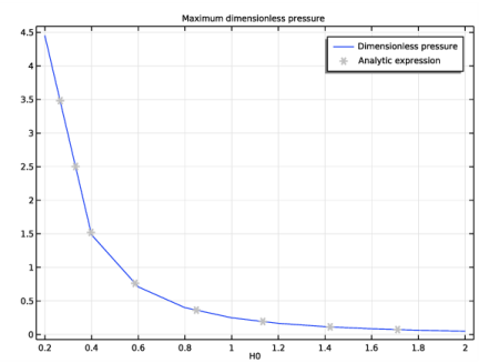
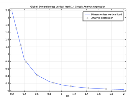
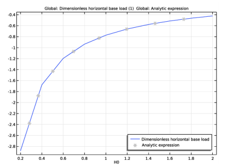
The results of the simulation are compared with the analytic expressions discussed above in Figure 2 to Figure 7. In all cases the agreement between COMSOL and the analytic results is excellent. The ratio H0 = h0/sh is a measure of the slope of the wall surface–for smaller values of H0 the slope is greater in relation to the exit height of the bearing. For smaller H0 larger pressures can be produced in the bearing and higher loads can be sustained by the bearing. The flow rate of gas through the bearing increases with increasing H0 as the flow tends toward a pure Couette flow, which produces no back pressure.

Figure 2: Nondimensional pressure vs distance along the bearing, plotted for different values of the film thickness ratio, H0=h0/sh. The computed results are shown as the continuous curves and the theoretical results as the gray symbols.

Figure 3: Nondimensional maximum pressure vs film thickness ratio, H0=h0/sh. The computed results are shown as the continuous curve and the theoretical result as the gray symbols.

Figure 4: Nondimensional flow rate vs film thickness ratio, H0=h0/sh. The computed results are shown as the continuous curve and the theoretical result as the gray symbols.

Figure 5: Nondimensional vertical load vs film thickness ratio, H0=h0/sh. The computed results are shown as the continuous curve and the theoretical result as the gray symbols.

Figure 6: Nondimensional horizontal wall load vs film thickness ratio, H0=h0/sh. The computed results are shown as the continuous curve and the theoretical result as the gray symbols.

Figure 7: Nondimensional horizontal base load vs film thickness ratio, H0=h0/sh. The computed results are shown as the continuous curve and the theoretical result as the gray symbols.

Reference

1. B.J. Hamrock, S.R. Schmid, and B.O. Jacobson, Fundamentals of Fluid Film Lubrication, Marcel Dekker, New York, 2004.

This example is based on the discussion entitled Fixed-Incline Slider Bearing in section 8.5 of the above reference.

CFD_Module/Thin-Film_Flow/slider_bearing_1d

Modeling Instructions

From the menu, choose .

New

In the window, click

Model Wizard

In the window, click

In the tree, select .

Click .

Click

In the tree, select .

Click

Global Definitions

Parameters 1

In the window, under click .

In the window for , locate the section.

In the table, enter the following settings:


Name	Expression	Value	Description
L	1[mm]	0.001 m	Bearing length
H0	0.1	0.1	Dimensionless height at end
sh	2[um]	2E-6 m	Additional height at start
h0	sh*H0	2E-7 m	Height at end
Vb	0.1[mm/s]	1E-4 m/s	Velocity of base
mu0	0.8[Pa*s]	0.8 Pa·s	Fluid viscosity
rho0	900[kg/m^3]	900 kg/m³	Fluid density

Geometry 1

Line Segment 1 (ls1)

In the toolbar, click

and choose .

In the window for , locate the section.

From the list, choose .

Locate the section. From the list, choose .

In the text field, type L.

Click

Definitions

Integration 1 (intop1)

In the toolbar, click

and choose .

In the window for , locate the section.

From the list, choose .

Select Boundary 1 only.

Integration 2 (intop2)

In the toolbar, click

and choose .

In the window for , locate the section.

From the list, choose .

Select Point 1 only.

Variables 1

In the toolbar, click

In the window for , locate the section.

In the table, enter the following settings:


Name	Expression	Unit	Description
hw	h0+sh*(1-x/L)	m	Wall height
Xd	x/L		Dimensionless length
Pd	pfilmsh^2/(mu0Vb*L)		Dimensionless pressure
Hd	hw/sh		Dimensionless height
Qd	2intop2(tffs.vavextffs.h)/(sh*Vb)		Dimensionless flow rate at inlet
VLd	-intop1(tffs.fwally)sh^2/(mu0Vb*L^2)		Dimensionless vertical load
HLwd	intop1(tffs.fwallx)sh/(mu0Vb*L)		Dimensionless horizontal wall load
HLbd	intop1(tffs.fbasex)sh/(mu0Vb*L)		Dimensionless horizontal base load
Pmaxan	3/(2H0(1+H0)(1+2H0))		Analytic maximum pressure
Qan	2H0(1+H0)/(1+2*H0)		Analytic dimensionless flow rate
VLan	6log((H0+1)/H0)-12/(1+2H0)		Analytic dimensionless vertical load
HLwan	4log((H0+1)/H0)-6/(1+2H0)		Analytic dimensionless horizontal wall load
HLban	4log(H0/(H0+1))+6/(1+2H0)		Analytic dimensionless horizontal base load