PDF

Dam Breaking on a Column, Shallow Water Equations
Introduction
Wave impact problems are important in engineering of structures, for example in locations where tsunamis are probable. Predicting the forces of waves acting on objects can be crucial for offshore structures and structures placed near water. If the structure is subjected to high waves, flooding must also be accounted for. One of the simplest, but widely used, systems of equations used to model this kind of problem are the shallow water equations.
This transient model solves the shallow water equations to model the impact of a water wave on a column. A body of water with a height of 0.3 m is initially contained behind a gate. At the start of the simulation, the gate is suddenly released and the body of water forms a wave moving toward the structure. After impacting, the water continues its forward movement until it is reflected from the wall of the tank and impinges the second time on the other side of the column. The pressure force on the column is computed and can be compared with the experimental results available in Ref. 1, and with the results obtained using the Two-Phase Flow, Level Set interface in the Dam Breaking on a Column, Level Set example.
Model Definition
The geometry and initial configuration of the experiment is depicted in Figure 1. A 1.60 m long, 0.61 m wide, and 0.60 m high tank was used. A 0.40 m long, 0.61 m wide, and 0.30 m high volume of water is initially contained behind a gate which is instantly released at the start of the simulation. A tall solid column with 0.12 m wide square base is placed inside the tank 0.50 m downstream of the wall and 0.25 m from one of the sidewalls. The experimental facility did not allow for a complete drainage of the tank so a thin layer of water of approximately 0.01 m is also accounted for.
Using the Shallow Water Equations, Time Explicit physics interface, the problem is solved in a 2D domain. The bottom of the tank is defined entering an expression for the bottom height in the Domain Properties feature. The lateral walls are modeled with the Wall feature. The initial height of the water is defined using the Initial Values feature. In this model the column is represented using the Wall feature. More complicated objects that could be flooded with water should be modeled entering an expression for the bottom height hb instead.
The physics interface provides variables to compute the pressure force acting on boundaries. In the shallow water equations the pressure is assumed to be hydrostatic
The pressure force per unit length on a boundary can be obtained integrating along h:
The components of the vector Fp can be accessed in 2D using the variables swe.Fpx and swe.Fpy. Note that these variables represent a force per unit length, the total force on a boundary is obtained integrating over the whole boundary.
Figure 1: Geometry and initial water configuration.
Results and Discussion
Figure 2 shows the position of the free surface at various times. After the release of the gate, the body of water collapses due to gravity and forms a wave moving toward the column. After impacting on the structure the wave front is torn so that its central part rides up the column’s upstream face. The sides of the wave rejoin in the wake downstream the structure and are reflected by the downstream wall of the tank. The wave is weakened after the reflection and impinges again on the column from the downstream side. The wave continues toward the upstream wall where it is reflected once more, but it is gradually decaying.
The net y-component of the pressure force acting on the column is plotted in Figure 3. The computed force captures the impact of the water on the front and back parts of the structure with maxima at t = 0.3 s and t = 1.4 s, respectively. Compared with the measured forces reported in Ref. 1, the agreement is good. The maximum and minimum values of the force are over predicted, but the trend of the force can be successfully captured using a simplified model as the shallow water equations.
Figure 2: Water free surface at t = 0.22 s, 0.38 s, 0.76 s, 1.44 s, 1.78 s, and 2.30 s.
Figure 3: Force in the y direction acting on the structure.
References
1. P.E. Raad and R. Bidoae, “The three-dimensional Eulerian-Lagrangian marker and micro cell method for the simulation of free surface flows,” J. Comput. Phys., vol. 203, pp. 668–699, 2005.
Application Library path: CFD_Module/Shallow_Water_Equations/dam_break_column_sw
Modeling Instructions
From the File menu, choose New.
New
In the New window, click  Model Wizard.
Model Wizard
1
In the Model Wizard window, click  2D.
2
In the Select Physics tree, select Fluid Flow>Shallow Water Equations>Shallow Water Equations, Time Explicit (swe).
3
Click Add.
4
Click  Study.
5
In the Select Study tree, select Preset Studies for Selected Physics Interfaces>Time Dependent.
6
Geometry 1
Rectangle 1 (r1)
1
In the Geometry toolbar, click  Rectangle.
2
In the Settings window for Rectangle, locate the Size and Shape section.
3
In the Width text field, type 0.61.
4
In the Height text field, type 1.6.
5
Click to expand the Layers section. In the table, enter the following settings:
Square 1 (sq1)
1
In the Geometry toolbar, click  Square.
2
In the Settings window for Square, locate the Size section.
3
In the Side length text field, type 0.12.
4
Locate the Position section. In the x text field, type 0.24.
5
In the y text field, type 0.9.
Difference 1 (dif1)
1
In the Geometry toolbar, click  Booleans and Partitions and choose Difference.
2
3
In the Settings window for Difference, locate the Difference section.
4
Find the Objects to subtract subsection. Click to select the  Activate Selection toggle button.
5
6
Click  Build All Objects.
Shallow Water Equations, Time Explicit (swe)
Initial Values 1
1
In the Model Builder window, under Component 1 (comp1)>Shallow Water Equations, Time Explicit (swe) click Initial Values 1.
2
In the Settings window for Initial Values, locate the Initial Values section.
3
In the h text field, type 0.01.
Initial Values 2
1
In the Physics toolbar, click  Domains and choose Initial Values.
2
3
In the Settings window for Initial Values, locate the Initial Values section.
4
In the h text field, type 0.3.
Definitions
Add a Boundary Probe to compute the pressure force acting on the column.
Boundary Probe 1 (bnd1)
1
In the Definitions toolbar, click  Probes and choose Boundary Probe.
2
In the Settings window for Boundary Probe, type Fp in the Variable name text field.
3
Locate the Probe Type section. From the Type list, choose Integral.
4
Locate the Source Selection section. From the Selection list, choose Manual.
5
Click  Clear Selection.
6
7
Locate the Expression section. In the Expression text field, type swe.Fpy.
8
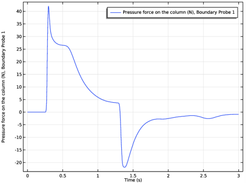
Select the Description check box.
9
In the associated text field, type Pressure force on the column.
Mesh 1
1
In the Model Builder window, under Component 1 (comp1) click Mesh 1.
2
In the Settings window for Mesh, locate the Physics-Controlled Mesh section.
3
From the Element size list, choose Finer.
4
Click  Build All.
Study 1
Step 2: Time Dependent
1
In the Model Builder window, under Study 1 click Step 2: Time Dependent.
2
In the Settings window for Time Dependent, locate the Study Settings section.
3
In the Output times text field, type range(0,0.01,3).
4
In the Study toolbar, click  Get Initial Value.
Results
Total Height (swe)
In the Model Builder window, expand the Total Height (swe) node.
Height Expression 1
1
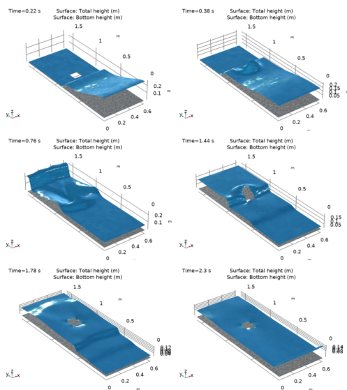
In the Model Builder window, expand the Results>Total Height (swe)>Total Height node, then click Height Expression 1.
2
In the Settings window for Height Expression, locate the Axis section.
3
Select the Scale factor check box.
Study 1
In the Study toolbar, click  Compute.
Results
Total Height (swe)
1
In the Settings window for 2D Plot Group, locate the Data section.
2
From the Time (s) list, choose 0.38.
3
In the Total Height (swe) toolbar, click  Plot.