PDF

Dam Breaking on a Column, Level Set
Introduction
Wave impact problems are important in engineering of structures, for example in locations where the event of tsunami is probable. Predicting the forces of waves acting on objects can be crucial for offshore structures and structures placed near water. If the structure is subjected to high waves, flooding must also be accounted for. One of the simplest and widely used ways used to model this kind of problems is the shallow water equation system.
In this transient study, the Two-Phase Flow, Level Set interface is used instead to model the impact of a water wave on a column. A body of water with a height of 0.3 m is initially contained behind a gate. At the onset of the simulation, the gate is suddenly released and the body of water forms a wave moving toward the structure. After impacting, the water continues forward movement until it is reflected at the wall of the tank and impinges second time on the column. The pressure force on the column is computed and can be compared with the experimental results available in Ref. 1 as well as with the results obtained using the Shallow Water Equations, Time Explicit interface in Dam Breaking on a Column, Shallow Water Equations.
Model Definition
The geometry and initial configuration of the experiment are depicted in Figure 1. A 1.60 m long, 0.61 m wide, and 0.60 m high tank is used. A 0.40 m long, 0.61 m wide, and 0.30 m high bulk of water is initially contained behind a gate which is instantly released at the simulation onset. A tall solid column with 0.12 m wide square base is placed inside the tank 0.50 m downstream of the gate and 0.25 m from one of the sidewalls. The experimental facility did not allow for a complete drainage of the tank and a thin layer of water of approximately 0.01 m has to also be accounted for.
The pressure force per unit length on a boundary can be obtained using an integration operator,
where Γ represents the front and back boundaries of the column.
Figure 1: Geometry and initial water configuration.
Results and Discussion
Figure 2 shows the position of the free surface at various times. After the release of the gate, the body of water collapses due to gravity and forms a wave moving toward the column. Upon impacting the structure, the wave is divided and its center part rides up the column’s upstream face. The sides of the wave front rejoin in the wake downstream the structure and later become reflected from the downstream wall of the tank. The wave is weakened after the reflection and impinges again on the downstream face of the column. The wave then continues toward the upstream wall, while slowly decaying.
The net y-component of the pressure force acting on the column is plotted in Figure 3. The computed force captures the impact of the evolving wave on the front and rear parts of the structure with maxima at t = 0.35 s and t = 1.5 s, respectively. Compared with the measured forces reported in Ref. 1, the agreement is good. The results are better than the ones obtained with the shallow water equations in Dam Breaking on a Column, Shallow Water Equations.
Figure 2: Water free surface at t = 0 s, 0.2 s, 0.5 s, 0.9 s, 1.5 s, and 1.7 s.
Figure 3: Force in the y direction acting on the structure.
Notes About the COMSOL Implementation
The present application uses the Block-Navier Stokes preconditioner instead of the default preconditioner for GMRES when solving the Navier-Stokes equations. This preconditioner can uncouple the pressure and velocity equations when solving, and may provide faster solutions for large time dependent models with incompressible flow and high Reynolds numbers (low viscosities).
Reference
1. P.E. Raad and R. Bidoae, “The three-dimensional Eulerian-Lagrangian marker and micro cell method for the simulation of free surface flows,” J. Comput. Phys., vol. 203, pp. 668–699, 2005.
Application Library path: CFD_Module/Multiphase_Flow/dam_break_column_ls
Modeling Instructions
From the File menu, choose New.
New
In the New window, click  Model Wizard.
Model Wizard
1
In the Model Wizard window, click  3D.
2
In the Select Physics tree, select Fluid Flow>Multiphase Flow>Two-Phase Flow, Level Set>Laminar Flow.
3
Click Add.
4
Click  Study.
5
In the Select Study tree, select Preset Studies for Selected Multiphysics>Time Dependent with Phase Initialization.
6
Geometry 1
Block 1 (blk1)
1
In the Geometry toolbar, click  Block.
2
In the Settings window for Block, locate the Size and Shape section.
3
In the Width text field, type 1.6.
4
In the Depth text field, type 0.61.
5
In the Height text field, type 0.6.
6
Click to expand the Layers section. In the table, enter the following settings:
Block 2 (blk2)
1
In the Geometry toolbar, click  Block.
2
In the Settings window for Block, locate the Size and Shape section.
3
In the Width text field, type 0.4.
4
In the Depth text field, type 0.61.
5
In the Height text field, type 0.3.
Block 3 (blk3)
1
In the Geometry toolbar, click  Block.
2
In the Settings window for Block, locate the Size and Shape section.
3
In the Width text field, type 0.12.
4
In the Depth text field, type 0.12.
5
In the Height text field, type 0.6.
6
Locate the Position section. In the x text field, type 0.9.
7
In the y text field, type 0.25.
8
Click  Build Selected.
Difference 1 (dif1)
1
In the Geometry toolbar, click  Booleans and Partitions and choose Difference.
2
3
In the Settings window for Difference, locate the Difference section.
4
Find the Objects to subtract subsection. Click to select the  Activate Selection toggle button.
5
6
Click  Build Selected.
Block 4 (blk4)
1
In the Model Builder window, under Component 1 (comp1)>Geometry 1 right-click Block 2 (blk2) and choose Duplicate.
2
In the Settings window for Block, click  Build Selected.
Difference 2 (dif2)
1
In the Geometry toolbar, click  Booleans and Partitions and choose Difference.
2
3
In the Settings window for Difference, locate the Difference section.
4
Find the Objects to subtract subsection. Click to select the  Activate Selection toggle button.
5
6
Click  Build Selected.
Split 1 (spl1)
1
In the Geometry toolbar, click  Conversions and choose Split.
2
3
In the Settings window for Split, click  Build Selected.
Union 1 (uni1)
1
In the Geometry toolbar, click  Booleans and Partitions and choose Union.
2
Select the objects blk4 and spl1(2) only.
3
In the Settings window for Union, locate the Union section.
4
Clear the Keep interior boundaries check box.
5
Click  Build All Objects.
Definitions
Integration 1 (intop1)
1
In the Definitions toolbar, click  Nonlocal Couplings and choose Integration.
2
In the Settings window for Integration, locate the Source Selection section.
3
From the Geometric entity level list, choose Boundary.
4
Click the  Wireframe Rendering button in the Graphics toolbar.
5
Global Variable Probe 1 (var1)
1
In the Definitions toolbar, click  Probes and choose Global Variable Probe.
2
In the Settings window for Global Variable Probe, type Fp in the Variable name text field.
3
Locate the Expression section. In the Expression text field, type intop1(p*spf.nxmesh).
4
Select the Description check box.
5
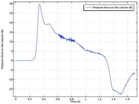
In the associated text field, type Pressure force on the column.
Add Material
1
In the Home toolbar, click  Add Material to open the Add Material window.
2
Go to the Add Material window.
3
In the tree, select Built-in>Water, liquid.
4
Right-click and choose Add to Component 1 (comp1).
5
6
Right-click and choose Add to Component 1 (comp1).
7
In the Home toolbar, click  Add Material to close the Add Material window.
Materials
Air (mat2)
1
Click the  Show More Options button in the Model Builder toolbar.
2
In the Show More Options dialog box, in the tree, select the check box for the node Physics>Advanced Physics Options.
3
Laminar Flow (spf)
1
In the Model Builder window, under Component 1 (comp1) click Laminar Flow (spf).
2
In the Settings window for Laminar Flow, locate the Physical Model section.
3
Select the Include gravity check box.
4
Click to expand the Advanced Settings section. Find the Linear solver subsection. Select the Use Block Navier-Stokes preconditioner in time dependent studies check box.
Pressure Point Constraint 1
1
In the Physics toolbar, click  Points and choose Pressure Point Constraint.
2
Level Set (ls)
Level Set Model 1
1
In the Model Builder window, under Component 1 (comp1)>Level Set (ls) click Level Set Model 1.
2
In the Settings window for Level Set Model, locate the Level Set Model section.
3
In the γ text field, type 10.
Initial Values, Fluid 2
1
In the Model Builder window, click Initial Values, Fluid 2.
2
Multiphysics
Two-Phase Flow, Level Set 1 (tpf1)
1
In the Model Builder window, under Component 1 (comp1)>Multiphysics click Two-Phase Flow, Level Set 1 (tpf1).
2
In the Settings window for Two-Phase Flow, Level Set, locate the Fluid 1 Properties section.
3
From the Fluid 1 list, choose Water, liquid (mat1).
4
Locate the Fluid 2 Properties section. From the Fluid 2 list, choose Air (mat2).
Wetted Wall 1 (ww1)
1
In the Model Builder window, click Wetted Wall 1 (ww1).
2
In the Settings window for Wetted Wall, locate the Boundary Selection section.
3
From the Selection list, choose All boundaries.
Mesh 1
1
In the Model Builder window, under Component 1 (comp1) click Mesh 1.
2
In the Settings window for Mesh, locate the Physics-Controlled Mesh section.
3
From the Element size list, choose Finer.
4
Click  Build All.
Study 1
Step 2: Time Dependent
1
In the Model Builder window, under Study 1 click Step 2: Time Dependent.
2
In the Settings window for Time Dependent, locate the Study Settings section.
3
In the Output times text field, type range(0,0.05,1.7).
Solution 1 (sol1)
1
In the Study toolbar, click  Show Default Solver.
2
In the Model Builder window, expand the Solution 1 (sol1) node.
3
In the Model Builder window, expand the Study 1>Solver Configurations>Solution 1 (sol1)>Dependent Variables 2 node, then click Velocity field (comp1.u).
4
In the Settings window for Field, locate the Scaling section.
5
From the Method list, choose Manual.
6
In the Scale text field, type 10.
7
In the Model Builder window, under Study 1>Solver Configurations>Solution 1 (sol1) click Time-Dependent Solver 1.
8
In the Settings window for Time-Dependent Solver, click to expand the Time Stepping section.
9
Find the Algebraic variable settings subsection. In the Fraction of initial step for Backward Euler text field, type 1.
10
In the Study toolbar, click  Get Initial Value.
Results
1
In the Model Builder window, click Results.
2
In the Settings window for Results, locate the Update of Results section.
3
Select the Only plot when requested check box.
Volume Fraction of Fluid 1 (ls)
1
In the Model Builder window, under Results click Volume Fraction of Fluid 1 (ls).
2
In the Settings window for 3D Plot Group, locate the Plot Settings section.
3
Clear the Plot dataset edges check box.
Slice 1
1
In the Model Builder window, expand the Volume Fraction of Fluid 1 (ls) node.
2
Right-click Results>Volume Fraction of Fluid 1 (ls)>Slice 1 and choose Delete. Click Yes to confirm.
Material Appearance 1
In the Model Builder window, right-click Isosurface 1 and choose Material Appearance.
Transparency 1
1
Right-click Isosurface 1 and choose Transparency.
2
In the Settings window for Transparency, locate the Transparency section.
3
Set the Transparency value to 0.15.
Surface 1
1
In the Model Builder window, right-click Volume Fraction of Fluid 1 (ls) and choose Surface.
2
In the Settings window for Surface, click Replace Expression in the upper-right corner of the Expression section. From the menu, choose Component 1 (comp1)>Level Set>ls.Vf1 - Volume fraction of fluid 1.
3
Click to expand the Range section. Select the Manual data range check box.
4
In the Minimum text field, type 0.5.
5
In the Maximum text field, type 1.
Selection 1
1
Right-click Surface 1 and choose Selection.
2
In the Settings window for Selection, locate the Selection section.
3
From the Selection list, choose All boundaries.
4
In the list, choose 6, 12, and 13.
5
Click  Remove from Selection.
Material Appearance 1
In the Model Builder window, right-click Surface 1 and choose Material Appearance.
Transparency 1
1
Right-click Surface 1 and choose Transparency.
2
In the Settings window for Transparency, locate the Transparency section.
3
Set the Transparency value to 0.15.
Surface 2
1
In the Model Builder window, right-click Volume Fraction of Fluid 1 (ls) and choose Surface.
2
In the Settings window for Surface, locate the Expression section.
3
In the Expression text field, type 1.
Selection 1
1
Right-click Surface 2 and choose Selection.
2
In the Settings window for Selection, locate the Selection section.
3
Click  Paste Selection.
4
In the Paste Selection dialog box, type 2, 3, 5, 10, 11, 15-24 in the Selection text field.
5
Material Appearance 1
1
In the Model Builder window, right-click Surface 2 and choose Material Appearance.
2
In the Settings window for Material Appearance, locate the Appearance section.
3
From the Appearance list, choose Custom.
4
From the Material type list, choose Steel (scratched).
5
In the Volume Fraction of Fluid 1 (ls) toolbar, click  Plot.
Study 1
In the Home toolbar, click  Compute.
Results
Probe Plot Group 4
1
In the Model Builder window, under Results click Probe Plot Group 4.
2
In the Probe Plot Group 4 toolbar, click  Plot.
Volume Fraction of Fluid 1 (ls)
1
In the Model Builder window, click Volume Fraction of Fluid 1 (ls).
2
In the Settings window for 3D Plot Group, locate the Data section.
3
From the Time (s) list, choose 0.9.
4
In the Volume Fraction of Fluid 1 (ls) toolbar, click  Plot.