Unsteady 3D Flow Past a Cylinder

Fluid flow past a cylinder is a common test case in computational fluid dynamics. The flow pattern is characterized by the Reynolds number which is defined as

where ρ is the density, Umean is the mean velocity of the free stream, D is the cylinder diameter, and μ is the dynamic viscosity.

The flow patterns around a cylinder in a free stream for different Reynolds numbers are shown in Ref. 1. At Re below 5, the flow remains attached to the cylinder. For Re between 5 and 15, steady wake vortices start forming on the downstream side of the cylinder. The wake becomes unsteady and forms a laminar vortex street for Re between 40 and 150.

Flow around a cylinder in a channel is even more complicated due to the effect of wall boundaries. Computer simulations of this problem at the intermediate Re regime (between 40 and 150) are challenging since they need to be 3D and time-dependent.

In this verification model, a benchmark problem of unsteady, incompressible 3D flow past a cylinder for Re = 100 during a period of 8 seconds is considered. The lift and drag coefficients are computed and are compared with those in Ref. 2.

Model Definition

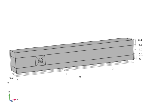
The geometry is a cylinder of radius R with the axis parallel to the z-axis, and placed at

, inside the box

. Figure 1 shows the geometry corresponding to R = 0.05 m , L = 2.5 m, H = 0.5 m, and xc = 0.5 m, yc = 0.2 m.

The fluid to be considered is incompressible and Newtonian with a kinematic viscosity of 10-3 m2/s. The inflow velocity profile varies in time according to

The lift and drag coefficients CD and CL are computed as functions of time,

where FD and FL are the drag and lift forces, and A is the projected area, A = 2RH.

Figure 1: The geometry is a cylinder placed inside a box.

The simulation is performed with a relatively coarse mesh with 7200 hexahedral elements shown in Figure 2. P2+P2 shape functions are chosen for the velocity and pressure to allow for better conservation and higher accuracy compared to P2+P1 and P1+P1. The generalized alpha method with automatic time stepping is chosen since it has less damping than the BDF method.

Figure 2: The relatively coarse mesh, with 7200 hexahedral elements, used in the simulation.

Results and Discussion

Figure 3 shows the flow pattern at t = 7.95 s, the last saved time before the inflow velocity returns to zero.

The lift and drag coefficients versus time are shown in Figure 4 and Figure 5 respectively. They capture the general shape of those published Ref. 2 quite well.

When the mesh size is reduced by a factor of 2, resulting in 57,600 elements, the computational time increases by a factor of 8 but the agreement with the current simulation is still excellent.

Figure 3: Computed velocity field at t = 7.95 s.

Figure 4: Lift coefficient versus time.

Figure 5: Drag coefficient versus time.

Notes About the COMSOL Implementation

The space discretization P2+P2 coupled with the generalized alpha time discretization works efficiently for this application. P2+P2 elements allow for a coarser mesh, better conservation, and more accuracy compared to P2+P1 and P1+P1 elements. The generalized alpha method has less damping than the BDF method. Automatic time-stepping works well and relatively large time steps can be used, and thus less computational time is needed compared to Ref. 2.

References

1. M. Van Dyke, An album of fluid motion, the Parabolic Press, ISBN 0-915760-03-7, 1982.

2. E. Bayraktar, O. Mierka, and S. Turek, “Benchmark Computation of 3D Laminar Flow Around a Cylinder with CFX, OpenFOAM and FeatFlow,” IJCSE, vol. 7, no. 3, pp. 253–266, 2012.

CFD_Module/Verification_Examples/cylinder_flow_3d_periodic

Modeling Instructions

From the menu, choose .

New

In the window, click

Model Wizard

In the window, click

In the tree, select .

Click .

Click

In the tree, select .

Click

Global Definitions

Parameters 1

In the window, under click .

In the window for , locate the section.

In the table, enter the following settings:


Name	Expression	Value	Description
U_mean	1[m/s]	1 m/s	Mean inflow velocity
rho	1[kg/m^3]	1 kg/m³	Density
mu	0.001[Pa*s]	0.001 Pa·s	Dynamic viscosity
H	0.41[m]	0.41 m	Height and Width
L	2.5[m]	2.5 m	Length
xc	0.5[m]	0.5 m	Cylinder x-pos
yc	0.2[m]	0.2 m	Cylinder y-pos
R	0.05[m]	0.05 m	Cylinder radius

Geometry 1

First, create the box [0, L]×[0, H]×[0, H].

Block 1 (blk1)

In the toolbar, click

In the window for , locate the section.

In the text field, type L.

In the text field, type H.

Next, create a smaller box around the cylinder. This box will be used later on in the meshing sequence.

Block 2 (blk2)

In the toolbar, click

In the window for , locate the section.

In the text field, type 4*R.

In the text field, type H.

Locate the section. In the text field, type xc-2*R.

In the text field, type yc-2*R.

Now, create the cylinder.

Cylinder 1 (cyl1)

In the toolbar, click

In the window for , locate the section.

In the text field, type R.

In the text field, type H.

Locate the section. In the text field, type xc.

In the text field, type yc.

Locate the section. In the text field, type 45.

In the toolbar, click

The following operations divide the flow domain into a number of subdomains. This way, a coarser mesh can be used far from the cylinder.

Line Segment 1 (ls1)

In the toolbar, click

and choose .

On the object , select Point 2 only.

In the window for , locate the section.

Find the subsection. Click to select the

toggle button.

On the object , select Point 5 only.

Line Segment 2 (ls2)

In the toolbar, click

and choose .

On the object , select Point 6 only.

In the window for , locate the section.

Find the subsection. Click to select the

toggle button.

On the object , select Point 7 only.

Line Segment 3 (ls3)

In the toolbar, click

and choose .

On the object , select Point 8 only.

In the window for , locate the section.

Find the subsection. Click to select the

toggle button.

On the object , select Point 8 only.

Line Segment 4 (ls4)

In the toolbar, click

and choose .

On the object , select Point 4 only.

In the window for , locate the section.

Find the subsection. Click to select the

toggle button.

On the object , select Point 6 only.

Click

Click the

button in the toolbar, and rotate the geometry to get a better view.

Block 3 (blk3)

In the toolbar, click

In the window for , locate the section.

In the text field, type L.

In the text field, type 2*R.

In the text field, type H.

Block 4 (blk4)

Right-click and choose .

In the window for , locate the section.

In the text field, type H-6*R.

Locate the section. In the text field, type 6*R.

Click

Now, create the final computational domain with a hollow cylinder.

Difference 1 (dif1)

In the toolbar, click

and choose .

Select the objects and only.

In the window for , locate the section.

Find the subsection. Click to select the

toggle button.

Select the object only.

In the toolbar, click

Click the

button in the toolbar. The geometry looks like the following image.

Laminar Flow (spf)

Click the

button in the toolbar.

In the dialog box, in the tree, select the check box for the node .

Click .

In the window, under click .

In the window for , click to expand the section.

Find the subsection. Clear the check box.

Click to expand the section. From the list, choose . P2+P2 is used because it is more conservative and more accurate than P2+P1 and P1+P1.

Fluid Properties 1

In the window, under click .

In the window for , locate the section.

From the ρ list, choose . In the associated text field, type rho.

From the μ list, choose . In the associated text field, type mu.

Inlet 1

In the toolbar, click

and choose .

Select Boundaries 1, 5, and 9 only.

In the window for , locate the section.

In the U0 text field, type 36*U_mean*z*y*(H-y)*(H-z)/H^4*sin(pi*t/8[s]).

Here, 1/[s] is used to make the input of sin() dimensionless.

Outlet 1

In the toolbar, click

and choose .

Select Boundaries 31–33 only.

Mesh 1

Use advanced operations such as Map and Sweep to create a hexahedral mesh.

Mapped 1

In the toolbar, click

and choose .

Size

In the window, click .

In the window for , locate the section.

From the list, choose .

Mapped 1

In the window, click .

Select Boundaries 17, 18, 20, and 25 only.

Distribution 1

Right-click and choose .

Select Edges 22, 24, 28, 32, 33, 36, 39, and 46 only.

In the window for , click

Distribution 2

Right-click and choose .

Select Edges 23 and 27 only.

In the window for , locate the section.

From the list, choose .

In the text field, type 2.

From the list, choose .

Distribution 3

Right-click and choose .

Select Edges 40 and 42 only.

In the window for , locate the section.

From the list, choose .

In the text field, type 2.

From the list, choose .

Click

Mapped 2

In the toolbar, click

and choose .

Select Boundaries 8 and 29 only.

Distribution 1

Right-click and choose .

Select Edges 9 and 56 only.

Distribution 2

In the window, right-click and choose .

Select Edges 10 and 15 only.

In the window for , locate the section.

From the list, choose .

In the text field, type 8.

In the text field, type 3.

From the list, choose .

Distribution 3

Right-click and choose .

Select Edges 47 and 50 only.

In the window for , locate the section.

From the list, choose .

In the text field, type 30.

In the text field, type 6.

From the list, choose .

Select the check box.

Mapped 3

In the toolbar, click

and choose .

Select Boundaries 4 and 12 only.

Distribution 1

Right-click and choose .

Select Edges 14 and 59 only.

In the window for , locate the section.

From the list, choose .

In the text field, type 4.

From the list, choose .

Distribution 2

In the window, right-click and choose .

Select Edges 4 and 53 only.

In the window for , locate the section.

From the list, choose .

In the text field, type 4.

From the list, choose .

Select the check box.

Distribution 3

Right-click and choose .

Select Edges 5 and 18 only.

In the window for , locate the section.

From the list, choose .

In the text field, type 43.

In the text field, type 1.6.

From the list, choose .

Swept 1

In the toolbar, click

Distribution 1

Right-click and choose .

In the window for , locate the section.

From the list, choose .

In the text field, type 10.

In the text field, type 4.

From the list, choose .

Select the check box.

Click

The mesh in Figure 2 is now generated.

Study 1

Step 1: Time Dependent

In the window, under click .

In the window for , locate the section.

In the text field, type range(0,0.05,8).

From the list, choose .

In the text field, type 0.001.

Solution 1 (sol1)

Choose the generalized alpha method for the time stepping. It has less damping than the BDF.

In the toolbar, click

In the window, expand the node.

In the window, under click .

In the window for , click to expand the section.

From the list, choose .

Select the check box.

In the associated text field, type 0.01.

From the list, choose .

In the toolbar, click

Evaluate the drag and lift coefficients.

Results

Surface 2

In the toolbar, click

and choose .

Select Boundaries 21–24 only.

Integral 1

In the toolbar, click

and choose .

In the window for , locate the section.

From the list, choose .

Point Evaluation 1

In the toolbar, click

In the window for , locate the section.

From the list, choose .

Locate the section. In the table, enter the following settings:


Expression	Unit	Description
-spf.T_stressy/(0.5spf.rho(U_mean)^2(2R*H))	1	Lift coefficient
-spf.T_stressx/(0.5spf.rho(U_mean)^2(2R*H))	1	Drag coefficient

Click

Table

Go to the window.

Click in the window toolbar.

Table

Go to the window.

Click in the window toolbar.

Plot the lift coefficient versus time as shown in Figure 4.

In the window, under click .

In the window for , locate the section.

From the list, choose .

In the list, select .

Results

Lift coefficient

In the window, under click .

In the window for , type Lift coefficient in the text field.

Locate the section. Select the check box.

In the associated text field, type c<sub>L</sub>.

Drag coefficient

Plot the drag coefficient versus time as shown in Figure 5.

Right-click and choose .

In the window for , type Drag coefficient in the text field.

Locate the section. In the text field, type c<sub>D</sub>.

Table Graph 1

In the window, expand the node, then click .

In the window for , locate the section.

In the list, select .

In the toolbar, click

Point Evaluation 1

Evaluate the maximum and minimum of the coefficients.

Point Evaluation 2

In the window, under right-click and choose .

In the window for , locate the section.

From the list, choose .

, then choose .

Go to the window.

Right-click and choose .

In the window for , locate the section.

Click to select row number 2 in the table.

Locate the section. From the list, choose .

Click

next to

, then choose .

Surface 3

In the toolbar, click

and choose .

Select Boundaries 2, 13, and 21–24 only.

Now, visualize the velocity field as shown in Figure 3.

Velocity (spf)

In the window, under click .

In the window for , locate the section.

Clear the check box.

Locate the section. Clear the check box.

Locate the section. From the list, choose . Since the inlet velocity vanishes at the final time step, the solution at t=7.95s is chosen for a better visualization of the streamlines.

Slice

Create a slice in the middle of the computational domain, parallel to the xy − plane to see the flow pattern more clearly.