PDF

Heterogeneous NMC Electrode
Introduction
In this example, time-dependent discharge and electrochemical impedance spectroscopy (EIS) simulations are made on a heterogeneous NMC (Nickel-Manganese-Cobalt) electrode structure.
A solid mechanics simulation is also made to study the effect of electrode expansion/contraction on the particle and binder stresses.
Model Definition
The model geometry is heterogeneous with regards to the electrode particles. However, since carbon filler, binder and electrolyte is treated as a single porous conductive binder domain following a partly homogenized approach as described in Ref. 1.
Figure 1 shows the model geometry which is generated from tomography data (Ref. 2) using a Model Method. The geometry consists of one separator domain, one domain representing the porous conductive binder, and number of particle domains. How the geometry is created is documented in the Heterogeneous Electrode Geometry Generation tutorial.
Figure 1: Model geometry.
Battery Model
The Lithium-Ion Battery interface is used to define the electrolyte mass and charge transport, as well as the charge transport of the electrode phase, using the Battery Material Library materials NMC 111, LiNi0.33Mn0.33Co0.33O2, Lithium Metal, Li, and LiPF6 in 3:7 EC:EMC to define the electrode and electrolyte properties, respectively.
The Transport of Diluted Species interface is used to define the diffusion of intercalated lithium within the electrode particles.
The electrochemically active electrolyte-electrode interfaces at the particle surfaces and the negative lithium foil electrode are defined using the Electrode Surface nodes in the Lithium-Ion Battery interface, using Electrode Reaction child-nodes to define the electrode kinetics. The surface intercalation flux of lithium at the particle surfaces are coupled to the electrochemical reactions using an Electrode Surface Coupling node in the Transport of Diluted Species interface.
The Electrode Surface boundary of the lithium metal electrode is grounded, whereas an Electrode Current boundary condition is used to set the total battery current on the current collector boundary of the NMC electrode.
The battery model is first used in a time-dependent study to perform a 2C discharge simulation from fully charged conditions.
In a second study, an EIS simulation is performed using an AC Impedance, Initial Values study at a 50% lithiation level of the NMC electrode.
Solid Mechanics Model
The local concentration of intercalated lithium in the particles is solved for during the discharge simulation. As the concentration levels in the particles change, the particles will either expand or contract. By coupling the strain of the particles to the local concentration levels, a stress-strain analysis of the binder and particles can be performed.
The Solid Mechanics interface is used to perform the stress-strain analysis, using separate Linear Elastic Material domain nodes for the separator, porous conductive binder and particle domains.
An Interpolation function is used to define the relation between strain and the intercalated lithium concentration of the NMC particles, as shown in Figure 2. This function is then used to define the strain in the particles using an Intercalation Strain sub-node to a Linear Elastic Material.
Figure 2: Strain vs intercalation level for NMC. The data was taken from Ref. 3.
Results and Discussion
Figure 3 shows the cell voltage during the 2C discharge.
Figure 3: Cell voltage during the 2C discharge.
Figure 4 shows the concentration of intercalated lithium in the particles, as well as the flux and concentration of lithium ions in the electrolyte halfway into the 2C discharge. During discharge, lithium dissolves in an anodic reaction at the lithium metal foil and is subsequently transported as ions toward the NMC particles. At the surface of the NMC materials, cathodic charge transfer occurs, and the formed lithium atoms intercalate and diffuse toward the interior of the particles.
Figure 4: Concentration of intercalated lithium in the particles, and lithium-ion flux streamlines, halfway into the 2C discharge. The color expression of the flux streamlines depict the lithium-ion concentration in the electrolyte.
Figure 5 shows the Nyquist plot from the EIS simulation. The half-circle stems from the charge transfer reaction at the NMC particles, whereas the approx 45º tail is related to the diffusion of intercalated lithium in the particles.
Figure 5: Nyquist plot of the impedance with respect to ground at the NMC current collector.
Figure 6 and Figure 7 show the stresses in the particles and porous conductive binder, respectively, halfway into the 2C discharge.
Figure 6: Particle stress halfway into the 2C discharge.
Figure 7: Binder stress halfway into the 2C discharge.
References
1. A. Schmidt, E. Ramani, T. Carraro, J. Joos, A. Weber, M. Kamlah, and E. Ivers-Tiffée, “Understanding Deviations between Spatially Resolved and Homogenized Cathode Models of Lithium-Ion Batteries”, Energy Technol. 2021, 2000881
2. M.Ebner, F. Geldmacher , F. Marone , M. Stampanoni, and V. Wood, “X-Ray Tomography of Porous, Transition Metal Oxide Based Lithium Ion Battery Electrodes,” Adv. Energy Mater., vol. 3, pp. 845–850, 2013. See also supporting information at https://onlinelibrary.wiley.com/doi/abs/10.1002/aenm.201200932
3. R. Koerver and others, “Chemo-mechanical expansion of lithium electrode materials — on the route to mechanically optimized all-solid-state batteries,” Energy Environ. Sci., vol. 11, pp. 2142–2158, 2018.
Application Library path: Battery_Design_Module/Batteries,_Heterogeneous/nmc_electrode_heterogeneous
Modeling Instructions
Root
Start by opening the file containing the heterogeneous electrode geometry.
Application Libraries
1
From the File menu, choose Application Libraries.
2
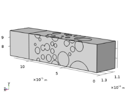
In the Application Libraries window, select Battery Design Module>Batteries, Heterogeneous>nmc_electrode_geometry in the tree.
3
Geometry 1
1
In the Model Builder window, expand the Component 1 (comp1) node.
2
Right-click Component 1 (comp1)>Geometry 1 and choose Build All.
3
Click the  Wireframe Rendering button in the Graphics toolbar.
4
Click the  Zoom Extents button in the Graphics toolbar.
Component 1 (comp1)
For setting up the physics, use the Lithium-Ion Battery interface and the Transport of Diluted Species interfaces.
Add Physics
1
In the Home toolbar, click  Add Physics to open the Add Physics window.
2
Go to the Add Physics window.
3
In the tree, select Electrochemistry>Batteries>Lithium-Ion Battery (liion).
4
Click Add to Component 1 in the window toolbar.
5
In the tree, select Chemical Species Transport>Transport of Diluted Species (tds).
6
Click Add to Component 1 in the window toolbar.
7
In the Home toolbar, click  Add Physics to close the Add Physics window.
Global Definitions
Add the electrode parameters from a text file.
Electrode Parameters
1
In the Home toolbar, click  Parameters and choose Add>Parameters.
2
In the Settings window for Parameters, locate the Parameters section.
3
Click  Load from File.
4
5
In the Label text field, type Electrode Parameters .
Materials
Add the materials for the electrodes and electrolyte from the material library.
Add Material
1
In the Home toolbar, click  Add Material to open the Add Material window.
2
Go to the Add Material window.
3
In the tree, select Battery>Electrodes>Lithium Metal, Li (Negative, Li-ion Battery).
4
Right-click and choose Add to Component 1 (comp1).
5
In the tree, select Battery>Electrodes>NMC 111, LiNi0.33Mn0.33Co0.33O2 (Positive, Li-ion Battery).
6
Right-click and choose Add to Component 1 (comp1).
7
In the tree, select Battery>Electrolytes>LiPF6 in 3:7 EC:EMC (Liquid, Li-ion Battery).
8
Right-click and choose Add to Component 1 (comp1).
9
In the Home toolbar, click  Add Material to close the Add Material window.
Materials
Lithium Metal, Li (Negative, Li-ion Battery) (mat1)
1
In the Settings window for Material, locate the Geometric Entity Selection section.
2
From the Geometric entity level list, choose Boundary.
3
From the Selection list, choose Lithium Foil.
NMC 111, LiNi0.33Mn0.33Co0.33O2 (Positive, Li-ion Battery) (mat2)
1
In the Model Builder window, click NMC 111, LiNi0.33Mn0.33Co0.33O2 (Positive, Li-ion Battery) (mat2).
2
In the Settings window for Material, locate the Geometric Entity Selection section.
3
From the Selection list, choose Particles.
LiPF6 in 3:7 EC:EMC (Liquid, Li-ion Battery) (mat3)
1
In the Model Builder window, click LiPF6 in 3:7 EC:EMC (Liquid, Li-ion Battery) (mat3).
2
In the Settings window for Material, locate the Geometric Entity Selection section.
3
From the Selection list, choose Separator + Binder.
Lithium-Ion Battery (liion)
1
In the Model Builder window, under Component 1 (comp1) click Lithium-Ion Battery (liion).
2
In the Settings window for Lithium-Ion Battery, locate the Domain Selection section.
3
From the Selection list, choose Separator + Binder.
4
Click to expand the Discretization section. Reduce the discretization to use linear elements for the battery interface. This will reduce the memory requirements for solving the model. Transport of Diluted species uses linear elements by default and needs not to be altered.
5
From the Electrolyte potential list, choose Linear.
6
From the Electrolyte salt concentration list, choose Linear.
7
From the Electric potential list, choose Linear.
Separator 1
1
In the Physics toolbar, click  Domains and choose Separator.
2
In the Settings window for Separator, locate the Domain Selection section.
3
From the Selection list, choose Separator.
4
Locate the Electrolyte Properties section. From the Electrolyte material list, choose LiPF6 in 3:7 EC:EMC (Liquid, Li-ion Battery) (mat3).
Porous Conductive Binder 1
1
In the Physics toolbar, click  Domains and choose Porous Conductive Binder.
2
In the Settings window for Porous Conductive Binder, locate the Domain Selection section.
3
From the Selection list, choose Porous Conductive Binder.
4
Locate the Electrolyte Properties section. From the Electrolyte material list, choose LiPF6 in 3:7 EC:EMC (Liquid, Li-ion Battery) (mat3).
5
Locate the Conductive Binder Properties section. From the σs list, choose User defined. In the associated text field, type sigma_s.
6
Locate the Porous Matrix Properties section. In the εs text field, type eps_s_b.
7
In the εl text field, type eps_l_b.
8
Locate the Effective Transport Parameter Correction section. From the Electrical conductivity list, choose No correction.
Internal Electrode Surface 1
Use the Internal Electrode Surface node to model the electrode-electrolyte interface between the particles and the porous conductive binder domain.
1
In the Physics toolbar, click  Boundaries and choose Internal Electrode Surface.
2
In the Settings window for Internal Electrode Surface, locate the Boundary Selection section.
3
From the Selection list, choose Particle Surfaces.
Electrode Reaction 1
Set the model input concentration, which is used by the active Material to calculate the equilibrium potential, to the concentration variable c solved for by the Transport of Diluted Species interface.
1
In the Model Builder window, click Electrode Reaction 1.
2
In the Settings window for Electrode Reaction, locate the Model Input section.
3
In the c text field, type c.
4
Locate the Material section. From the Material list, choose NMC 111, LiNi0.33Mn0.33Co0.33O2 (Positive, Li-ion Battery) (mat2).
5
Locate the Electrode Kinetics section. From the Kinetics expression type list, choose Lithium insertion.
6
In the i0,ref(T) text field, type i0_ref_NMC.
Electrode Surface 1
Use an Electrode Surface node to model the external lithium foil electrode.
1
In the Physics toolbar, click  Boundaries and choose Electrode Surface.
2
In the Settings window for Electrode Surface, locate the Boundary Selection section.
3
From the Selection list, choose Lithium Foil.
Electrode Reaction 1
1
In the Model Builder window, click Electrode Reaction 1.
2
In the Settings window for Electrode Reaction, locate the Electrode Kinetics section.
3
In the i0,ref(T) text field, type i0_ref_Li.
The Electrode Surface node is grounded by default. Use an Electrode Current node to define the cell current at the positive current collector boundary.
Electrode Current 1
1
In the Physics toolbar, click  Boundaries and choose Electrode Current.
2
In the Settings window for Electrode Current, locate the Boundary Selection section.
3
From the Selection list, choose NMC Current Collector.
4
Locate the Electrode Current section. In the Is,total text field, type -I_1C*C_rate.
Set the initial values for the electric potential, both on the boundary and in the domain.
5
In the φs,bnd,init text field, type mat2.elpot.Eeq_int1(cs0/csmax).
Initial Values 1
1
In the Model Builder window, click Initial Values 1.
2
In the Settings window for Initial Values, locate the Initial Values section.
3
In the phis text field, type mat2.elpot.Eeq_int1(cs0/csmax).
Transport of Diluted Species (tds)
Now define the diffusion of intercalated lithium in the particles.
1
In the Model Builder window, under Component 1 (comp1) click Transport of Diluted Species (tds).
2
In the Settings window for Transport of Diluted Species, locate the Domain Selection section.
3
From the Selection list, choose Particles.
4
Locate the Transport Mechanisms section. Clear the Convection check box.
Transport Properties 1
1
In the Model Builder window, under Component 1 (comp1)>Transport of Diluted Species (tds) click Transport Properties 1.
2
In the Settings window for Transport Properties, locate the Diffusion section.
3
From the Material list, choose NMC 111, LiNi0.33Mn0.33Co0.33O2 (Positive, Li-ion Battery) (mat2).
4
From the Dc list, choose Basic (def).
Initial Values 1
1
In the Model Builder window, click Initial Values 1.
2
In the Settings window for Initial Values, locate the Initial Values section.
3
In the c text field, type cs0.
Electrode Surface Coupling 1
1
In the Physics toolbar, click  Boundaries and choose Electrode Surface Coupling.
2
In the Settings window for Electrode Surface Coupling, locate the Boundary Selection section.
3
From the Selection list, choose Particle Surfaces.
Reaction Coefficients 1
1
In the Model Builder window, expand the Electrode Surface Coupling 1 node, then click Reaction Coefficients 1.
2
In the Settings window for Reaction Coefficients, locate the Model Inputs section.
3
From the iloc list, choose Local current density, Electrode Reaction 1 (liion/bei1/er1).
4
Locate the Stoichiometric Coefficients section. In the νc text field, type 1.
Definitions
Global Variable Probe - E cell
Add a probe for the cell voltage. The probe variable value will be stored in a table for every time step taken by the time-dependent solver.
1
In the Definitions toolbar, click  Probes and choose Global Variable Probe.
2
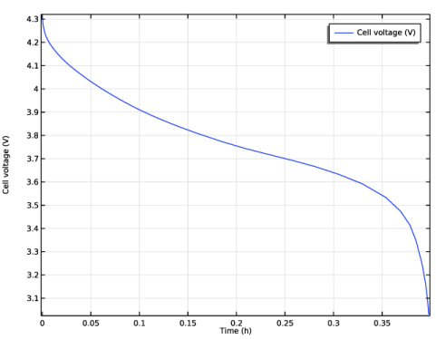
In the Settings window for Global Variable Probe, type Global Variable Probe - E cell in the Label text field.
3
Locate the Expression section. In the Expression text field, type liion.phis0_ec1.
4
Select the Description check box.
5
Mesh 1
1
In the Model Builder window, under Component 1 (comp1) click Mesh 1.
2
In the Settings window for Mesh, locate the Sequence Type section.
3
From the list, choose User-controlled mesh.
Size
1
In the Model Builder window, under Component 1 (comp1)>Mesh 1 click Size.
2
In the Settings window for Size, click to expand the Element Size Parameters section.
3
In the Maximum element size text field, type hmax.
4
In the Minimum element size text field, type hmin.
5
Click  Build All.
Add Study
1
In the Home toolbar, click  Add Study to open the Add Study window.
2
Go to the Add Study window.
3
Find the Studies subsection. In the Select Study tree, select Preset Studies for Selected Physics Interfaces>Lithium-Ion Battery>Time Dependent with Initialization.
4
Click Add Study in the window toolbar.
5
In the Home toolbar, click  Add Study to close the Add Study window.
Study 1 - Battery Discharge
1
In the Model Builder window, click Study 1.
2
In the Settings window for Study, type Study 1 - Battery Discharge in the Label text field.
Step 1: Current Distribution Initialization
1
In the Model Builder window, under Study 1 - Battery Discharge click Step 1: Current Distribution Initialization.
2
In the Settings window for Current Distribution Initialization, locate the Study Settings section.
3
From the Current distribution type list, choose Secondary.
4
Locate the Physics and Variables Selection section. In the table, clear the Solve for check box for Transport of Diluted Species (tds).
Step 2: Time Dependent
1
In the Model Builder window, click Step 2: Time Dependent.
2
In the Settings window for Time Dependent, locate the Study Settings section.
3
From the Time unit list, choose h.
4
In the Output times text field, type 0 0.1/C_rate 0.5/C_rate 0.9/C_rate.
Solution 1 (sol1)
1
In the Study toolbar, click  Show Default Solver.
Add a stop condition to define a cut-off voltage while discharging.
2
In the Model Builder window, expand the Solution 1 (sol1) node.
3
Right-click Study 1 - Battery Discharge>Solver Configurations>Solution 1 (sol1)>Time-Dependent Solver 1 and choose Stop Condition.
4
In the Settings window for Stop Condition, locate the Stop Expressions section.
5
6
7
Locate the Output at Stop section. Clear the Add warning check box.
Step 2: Time Dependent
1
In the Model Builder window, under Study 1 - Battery Discharge click Step 2: Time Dependent.
2
In the Settings window for Time Dependent, click to expand the Results While Solving section.
3
From the Probes list, choose Manual.
Solution 1 (sol1)
Place the electrolyte concentration dependent variable in a separate segregrated group. This will decrease the memory requirements of the solver.
1
In the Model Builder window, expand the Study 1 - Battery Discharge>Solver Configurations>Solution 1 (sol1)>Time-Dependent Solver 1>Segregated 1 node.
2
Right-click Study 1 - Battery Discharge>Solver Configurations>Solution 1 (sol1)>Time-Dependent Solver 1>Segregated 1 and choose Segregated Step.
3
In the Settings window for Segregated Step, locate the General section.
4
In the Variables list, select Electrolyte salt concentration (comp1.cl).
5
Under Variables, click  Delete.
6
In the Model Builder window, under Study 1 - Battery Discharge>Solver Configurations>Solution 1 (sol1)>Time-Dependent Solver 1>Segregated 1 click Segregated Step 3.
7
In the Settings window for Segregated Step, locate the General section.
8
Under Variables, click  Add.
9
In the Add dialog box, select Electrolyte salt concentration (comp1.cl) in the Variables list.
10
11
In the Settings window for Segregated Step, locate the General section.
12
From the Linear solver list, choose Direct, concentrations (tds).
13
In the Model Builder window, click Study 1 - Battery Discharge.
14
In the Settings window for Study, locate the Study Settings section.
15
Clear the Generate default plots check box.
16
In the Study toolbar, click  Compute.
Results
The probe plot is automatically generated as shown in (Figure 3).
Discharge voltage
1
In the Model Builder window, under Results click Probe Plot Group 1.
2
In the Settings window for 1D Plot Group, type Discharge voltage in the Label text field.
3
In the Discharge voltage toolbar, click  Plot.
Solid Lithium Concentration and Lithium Ion Flux
1
In the Home toolbar, click  Add Plot Group and choose 3D Plot Group.
Start plotting the concentration and the flux for the lithium ion in the heterogeneous electrode. (Figure 4).
2
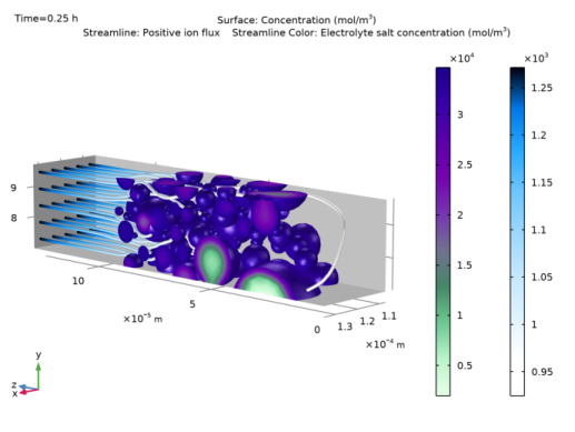
In the Settings window for 3D Plot Group, type Solid Lithium Concentration and Lithium Ion Flux in the Label text field.
3
Locate the Data section. From the Time (h) list, choose 0.25.
4
Locate the Plot Settings section. Clear the Plot dataset edges check box.
Surface 1
1
Right-click Solid Lithium Concentration and Lithium Ion Flux and choose Surface.
2
In the Settings window for Surface, locate the Expression section.
3
In the Expression text field, type c.
4
Locate the Coloring and Style section. From the Color table list, choose AuroraBorealis.
Streamline 1
1
In the Model Builder window, right-click Solid Lithium Concentration and Lithium Ion Flux and choose Streamline.
2
In the Settings window for Streamline, click Replace Expression in the upper-right corner of the Expression section. From the menu, choose Component 1 (comp1)>Lithium-Ion Battery>liion.Nposx,...,liion.Nposz - Positive ion flux.
3
Locate the Streamline Positioning section. In the Number text field, type 25.
4
Locate the Selection section. From the Selection list, choose Lithium Foil.
5
Locate the Coloring and Style section. Find the Line style subsection. From the Type list, choose Tube.
Color Expression 1
1
Right-click Streamline 1 and choose Color Expression.
2
In the Settings window for Color Expression, locate the Expression section.
3
In the Expression text field, type cl.
4
Click to expand the Title section. From the Title type list, choose Automatic.
5
Locate the Coloring and Style section. From the Color table list, choose JupiterAuroraBorealis.
6
From the Color table transformation list, choose Reverse.
Surface 2
1
In the Model Builder window, right-click Solid Lithium Concentration and Lithium Ion Flux and choose Surface.
2
In the Settings window for Surface, locate the Expression section.
3
In the Expression text field, type 1.
4
Click to expand the Title section. From the Title type list, choose None.
5
Locate the Coloring and Style section. From the Coloring list, choose Uniform.
6
From the Color list, choose Gray.
Selection 1
1
Right-click Surface 2 and choose Selection.
2
3
In the Solid Lithium Concentration and Lithium Ion Flux toolbar, click  Plot.
4
Click the  Zoom Extents button in the Graphics toolbar.
Lithium-Ion Battery (liion)
Now start setting up the model for the EIS simulation.
Electrode Current 1
Add a harmonic perturbation to perturb the current signal around the stationary value, which is zero current at open circuit in this case.
1
In the Model Builder window, under Component 1 (comp1)>Lithium-Ion Battery (liion) click Electrode Current 1.
Harmonic Perturbation 1
1
In the Physics toolbar, click  Attributes and choose Harmonic Perturbation.
2
In the Settings window for Harmonic Perturbation, locate the Harmonic Perturbation section.
3
In the ΔIs,total text field, type I_1C/100.
Add a double layer capacitance at the NMC surface.
Internal Electrode Surface 1
In the Model Builder window, under Component 1 (comp1)>Lithium-Ion Battery (liion) click Internal Electrode Surface 1.
Double Layer Capacitance 1
1
In the Physics toolbar, click  Attributes and choose Double Layer Capacitance.
2
In the Settings window for Double Layer Capacitance, locate the Double Layer Capacitance section.
3
In the Cdl text field, type C_dl_NMC.
4
Locate the Stoichiometric Coefficient section. In the νLi+ text field, type -1.
Global Definitions
Electrode Parameters
Modify the initial state of charge to 50 % lithiation before setting up the EIS study.
1
In the Model Builder window, under Global Definitions click Electrode Parameters.
2
In the Settings window for Parameters, locate the Parameters section.
3
Add Study
1
In the Home toolbar, click  Add Study to open the Add Study window.
2
Go to the Add Study window.
3
Find the Studies subsection. In the Select Study tree, select Empty Study.
4
Click Add Study in the window toolbar.
5
In the Home toolbar, click  Add Study to close the Add Study window.
Study 2 - EIS
In the Settings window for Study, type Study 2 - EIS in the Label text field.
Frequency Domain Perturbation
1
In the Study toolbar, click  Study Steps and choose Frequency Domain>Frequency Domain Perturbation.
2
In the Settings window for Frequency Domain Perturbation, locate the Study Settings section.
3
In the Frequencies text field, type 10^range(-2.6,0.2,5).
4
Click to expand the Results While Solving section. From the Probes list, choose None.
5
In the Model Builder window, collapse the Study 2 - EIS node.
6
In the Study toolbar, click  Compute.
Results
Impedance with Respect to Ground, Nyquist (liion)
1
In the Impedance with Respect to Ground, Nyquist (liion) toolbar, click  Plot.
2
Click the  Zoom Extents button in the Graphics toolbar.
Global Definitions
Solid Mechanics Parameters
Now set up the stress-strain model in the particles using the Solid Mechanics interface. Start by importing the parameters for the solid mechanics model.
1
In the Home toolbar, click  Parameters and choose Add>Parameters.
2
In the Settings window for Parameters, type Solid Mechanics Parameters in the Label text field.
3
Locate the Parameters section. Click  Load from File.
4
Add Physics
1
In the Home toolbar, click  Add Physics to open the Add Physics window.
2
Go to the Add Physics window.
3
In the tree, select Structural Mechanics>Solid Mechanics (solid).
4
Click Add to Component 1 in the window toolbar.
5
In the Home toolbar, click  Add Physics to close the Add Physics window.
Solid Mechanics (solid)
Linear Elastic Material 1
1
In the Model Builder window, under Component 1 (comp1)>Solid Mechanics (solid) click Linear Elastic Material 1.
2
In the Settings window for Linear Elastic Material, locate the Linear Elastic Material section.
3
From the E list, choose User defined. In the associated text field, type E_separator.
4
From the ν list, choose User defined. In the associated text field, type nu_separator.
5
From the ρ list, choose User defined. In the associated text field, type rho_separator.
Linear Elastic Material - Binder
1
In the Physics toolbar, click  Domains and choose Linear Elastic Material.
2
In the Settings window for Linear Elastic Material, type Linear Elastic Material - Binder in the Label text field.
3
Locate the Domain Selection section. From the Selection list, choose Porous Conductive Binder.
4
Locate the Linear Elastic Material section. From the E list, choose User defined. In the associated text field, type E_binder.
5
From the ν list, choose User defined. In the associated text field, type nu_binder.
6
From the ρ list, choose User defined. In the associated text field, type rho_binder.
Linear Elastic Material 3
1
In the Physics toolbar, click  Domains and choose Linear Elastic Material.
The strain in the particles depends on the concentration of intercalated lithium. First inspect the volumetric strain vs the lithiation level function, defined in the NMC material.
Materials
NMC 111, LiNi0.33Mn0.33Co0.33O2 (Positive, Li-ion Battery) (mat2)
In the Model Builder window, expand the NMC 111, LiNi0.33Mn0.33Co0.33O2 (Positive, Li-ion Battery) (mat2) node.
Interpolation 1 (dVOLdSOL)
1
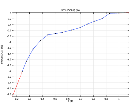
In the Model Builder window, expand the Component 1 (comp1)>Materials>NMC 111, LiNi0.33Mn0.33Co0.33O2 (Positive, Li-ion Battery) (mat2)>Intercalation strain (IntercalationStrain) node, then click Interpolation 1 (dVOLdSOL).
2
In the Settings window for Interpolation, click  Plot.
The function plot is shown in Figure 2.
Solid Mechanics (solid)
Linear Elastic Material - Particles
1
In the Model Builder window, under Component 1 (comp1)>Solid Mechanics (solid) click Linear Elastic Material 3.
2
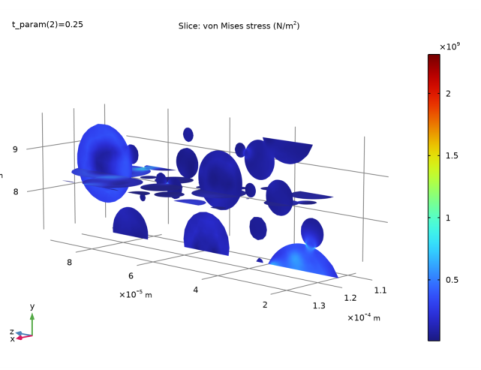
In the Settings window for Linear Elastic Material, type Linear Elastic Material - Particles in the Label text field.
3
Locate the Domain Selection section. From the Selection list, choose Particles.
4
Locate the Linear Elastic Material section. From the ρ list, choose User defined. In the associated text field, type rho_NMC.
Intercalation Strain 1
1
In the Physics toolbar, click  Attributes and choose Intercalation Strain.
The volumetric strain is taken From material by default. Couple the strain to the concentration solved for by the Transport of Diluted Species interface as follows:
2
In the Settings window for Intercalation Strain, locate the Model Input section.
3
From the c list, choose Concentration (tds).
Roller 1
1
In the Physics toolbar, click  Boundaries and choose Roller.
2
In the Settings window for Roller, locate the Boundary Selection section.
3
From the Selection list, choose All External Boundaries.
Add Study
1
In the Home toolbar, click  Add Study to open the Add Study window.
2
Go to the Add Study window.
3
Find the Studies subsection. In the Select Study tree, select General Studies>Stationary.
4
Click Add Study in the window toolbar.
5
In the Home toolbar, click  Add Study to close the Add Study window.
Study 3 - Solid Mechanics
1
In the Model Builder window, click Study 3.
2
In the Settings window for Study, type Study 3 - Solid Mechanics in the Label text field.
3
Locate the Study Settings section. Clear the Generate default plots check box.
Parametric Sweep
1
In the Study toolbar, click  Parametric Sweep.
2
In the Settings window for Parametric Sweep, locate the Study Settings section.
3
4
5
Locate the Output While Solving section. From the Probes list, choose None.
Stationary - Solid Mechanics
1
In the Model Builder window, click Step 1: Stationary.
2
In the Settings window for Stationary, type Stationary - Solid Mechanics in the Label text field.
3
Locate the Physics and Variables Selection section. In the table, clear the Solve for check boxes for Lithium-Ion Battery (liion) and Transport of Diluted Species (tds).
4
Click to expand the Values of Dependent Variables section. Find the Values of variables not solved for subsection. From the Settings list, choose User controlled.
5
From the Method list, choose Solution.
6
From the Study list, choose Study 1 - Battery Discharge, Time Dependent.
7
From the Time (h) list, choose Interpolated.
8
In the Time text field, type t_param.
Solution 4 (sol4)
1
In the Study toolbar, click  Show Default Solver.
2
In the Model Builder window, expand the Solution 4 (sol4) node.
By enabling the iterative solver, the memory requirements are reduced.
3
In the Model Builder window, expand the Study 3 - Solid Mechanics>Solver Configurations>Solution 4 (sol4)>Stationary Solver 1 node.
4
Right-click Study 3 - Solid Mechanics>Solver Configurations>Solution 4 (sol4)>Stationary Solver 1>Suggested Iterative Solver (solid) and choose Enable.
5
In the Study toolbar, click  Compute.
Results
Stress, Particles
1
In the Home toolbar, click  Add Plot Group and choose 3D Plot Group.
2
In the Settings window for 3D Plot Group, type Stress, Particles in the Label text field.
3
Locate the Data section. From the Dataset list, choose Study 3 - Solid Mechanics/Parametric Solutions 1 (sol5).
4
From the Parameter value (t_param) list, choose 0.25.
5
Locate the Plot Settings section. Clear the Plot dataset edges check box.
Slice 1
1
Right-click Stress, Particles and choose Slice.
2
In the Settings window for Slice, locate the Expression section.
3
In the Expression text field, type solid.mises.
4
Locate the Plane Data section. From the Plane list, choose ZX-planes.
5
In the Planes text field, type 1.
Selection 1
1
Right-click Slice 1 and choose Selection.
2
In the Settings window for Selection, locate the Selection section.
3
From the Selection list, choose Particles.
4
In the Stress, Particles toolbar, click  Plot.
Slice 2
1
In the Model Builder window, under Results>Stress, Particles right-click Slice 1 and choose Duplicate.
2
In the Settings window for Slice, locate the Plane Data section.
3
From the Plane list, choose YZ-planes.
4
In the Planes text field, type 1.
5
Click to expand the Inherit Style section. From the Plot list, choose Slice 1.
6
Click to expand the Title section. From the Title type list, choose None.
7
In the Stress, Particles toolbar, click  Plot.
8
Click the  Zoom Extents button in the Graphics toolbar.
This plot visualizes the stress in the particles. (Figure 6).
Stress, Binder
1
In the Model Builder window, right-click Stress, Particles and choose Duplicate.
2
In the Settings window for 3D Plot Group, type Stress, Binder in the Label text field.
Slice 1
In the Model Builder window, expand the Stress, Binder node.
Selection 1
1
In the Model Builder window, expand the Slice 1 node, then click Selection 1.
2
In the Settings window for Selection, locate the Selection section.
3
From the Selection list, choose Porous Conductive Binder.
Selection 1
1
In the Model Builder window, expand the Results>Stress, Binder>Slice 2 node, then click Selection 1.
2
In the Settings window for Selection, locate the Selection section.
3
From the Selection list, choose Porous Conductive Binder.
4
In the Stress, Binder toolbar, click  Plot.
5
Click the  Zoom Extents button in the Graphics toolbar.
This plots visualizes the stress in the binder domain. (Figure 7).