|
|
|


|
1
|
|
2
|
|
3
|
Click Add.
|
|
4
|
|
5
|
Click Add.
|
|
6
|
Click
|
|
7
|
|
8
|
Click
|
|
1
|
|
2
|
Browse to the model’s Application Libraries folder and double-click the file li_battery_thermal_2d_axi_geom_sequence.mph.
|
|
3
|
|
4
|
|
1
|
|
2
|
|
3
|
|
4
|
Browse to the model’s Application Libraries folder and double-click the file li_battery_thermal_2d_axi_parameters.txt.
|
|
1
|
|
2
|
|
3
|
|
4
|
|
1
|
|
2
|
|
1
|
|
2
|
|
3
|
|
4
|
|
5
|
|
6
|
|
1
|
|
2
|
|
3
|
|
4
|
|
1
|
|
2
|
|
3
|
|
4
|
|
1
|
|
2
|
|
3
|
|
4
|
|
5
|
|
1
|
|
2
|
|
1
|
|
2
|
|
3
|
|
4
|
|
5
|
|
6
|
|
1
|
In the Model Builder window, under Component 1 (comp1)>Lumped Battery (lb) click Cell Equilibrium Potential 1.
|
|
2
|
|
3
|
|
4
|
|
5
|
Browse to the model’s Application Libraries folder and double-click the file li_battery_thermal_2d_axi_E_OCP_data.txt.
|
|
6
|
|
7
|
|
8
|
Browse to the model’s Application Libraries folder and double-click the file li_battery_thermal_2d_axi_dEdT_data.txt.
|
|
1
|
|
2
|
|
3
|
|
4
|
|
5
|
Locate the Concentration Overpotential section. Select the Include concentration overpotential check box.
|
|
6
|
|
1
|
|
2
|
|
3
|
|
4
|
Locate the Heat Conduction, Solid section. From the k list, choose User defined. From the list, choose Diagonal.
|
|
5
|
In the k table, enter the following settings:
|
|
6
|
Locate the Thermodynamics, Solid section. From the ρ list, choose User defined. In the associated text field, type rho_batt.
|
|
7
|
|
1
|
|
2
|
|
3
|
|
4
|
Locate the Heat Conduction, Solid section. From the k list, choose User defined. In the associated text field, type kT_sep.
|
|
5
|
Locate the Thermodynamics, Solid section. From the ρ list, choose User defined. In the associated text field, type rho_sep.
|
|
6
|
|
1
|
|
3
|
|
4
|
|
5
|
|
6
|
|
1
|
|
2
|
|
3
|
|
1
|
|
2
|
|
3
|
|
4
|
|
1
|
|
2
|
|
3
|
|
4
|
|
5
|
|
1
|
|
2
|
|
3
|
|
4
|
|
5
|
|
1
|
|
2
|
|
1
|
|
2
|
|
3
|
|
4
|
|
5
|
|
1
|
|
2
|
|
3
|
|
4
|
|
5
|
|
6
|
|
1
|
|
2
|
|
3
|
|
4
|
|
5
|
|
6
|
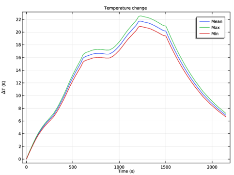
In the associated text field, type \DELTA T (K).
|
|
1
|
|
2
|
|
3
|
|
1
|
|
2
|
|
1
|
|
2
|
|
3
|
|
4
|
Browse to the model’s Application Libraries folder and double-click the file li_battery_thermal_2d_axi_geom_sequence_parameters.txt.
|
|
1
|
|
2
|
|
3
|
|
4
|
|
5
|
Click to expand the Layers section. In the table, enter the following settings:
|
|
1
|
|
2
|
|
3
|
|
4
|
|
5
|
Locate the Layers section. In the table, enter the following settings:
|
|
6
|
|
7
|
|
8
|
|
1
|
|
2
|
|
3
|
|
4
|
|
5
|
Click OK.
|
|
1
|
|
2
|
|
3
|
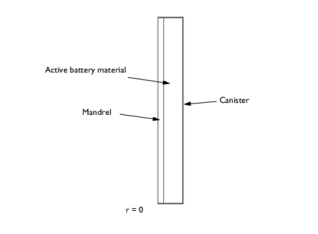
On the object mce1, select Domain 1 only.
|
|
1
|
|
2
|
In the Settings window for Explicit Selection, type Active Battery Material in the Label text field.
|
|
3
|
On the object mce1, select Domain 3 only.
|
|
1
|
|
2
|
|
3
|
On the object mce1, select Domain 2 only.
|