PDF

Single Particle Model of a Lithium-Ion Battery
Introduction
The single particle model for a lithium-ion battery is a simplification of the 1D model formulation (see the 1D Isothermal Lithium-Ion Battery model example), subject to a few assumptions. This model example demonstrates the Single Particle Battery interface for studying the discharge of a lithium-ion battery. The model is isothermal and is set in 0D space dimension. The voltage profiles are compared with the corresponding 1D formulation for a range of discharge currents.
In the single particle model formulation (Ref. 1and Ref. 2), the local potential and concentration gradients in the solution (electrolyte) phase are ignored and accounted for using a lumped solution resistance term. Similarly, the potential gradients in the solid phase of the electrodes are also neglected. Additionally, the porous electrode is treated as a large number of single particles all of them being subjected to the same conditions, since the reaction current distribution across the porous electrodes is assumed to be uniform. The single particle formulation accounts for solid diffusion in the electrode particles and the intercalation reaction kinetics.
The assumptions in the single particle formulation are typically valid for low-medium applied current densities. Additionally, the validity of the assumptions and the applicability of the model also depends on the parameters values and electrode-electrolyte chemistry used in the model. For example, the assumptions would be reasonable for thin electrodes, highly conductive electrodes, and so forth.
The single particle model formulation can be used for parameter estimation studies (kinetic and transport parameters) by comparing with experimental data. Additionally, it can be used instead of the more elaborate 1D formulation in computationally expensive scenarios such as thermal simulations, cycling behavior, battery pack simulations, and so forth.
Model Definition
The Single Particle Battery interface accounts for solid diffusion in the electrode particles and the intercalation reaction kinetics. The ohmic potential drop in the electrolyte is included using a lumped solution resistance term.
In this model example, the intercalation particles in the porous electrode are assumed to be spherical particles of identical size. Diffusion of lithium in the active material particles in the positive and negative electrodes is described by Fick’s second law. The intercalation reaction kinetics is expressed using the lithium insertion kinetics.
This model example is set in 0D space dimension for studying a galvanostatic operation for different discharge currents ranging from 0.1 C to 2 C, and a charge-discharge cycling operation at 1 C. The cell capacity is specified though fractional volumes of the positive and negative electrodes in the battery. The individual electrode operational state-of-charges are used to specify the initial charge distribution in the battery.
Model parameters
All the model parameters required by the single particle model are identical to the parameters used in the 1D Isothermal Lithium-Ion Battery model, for the purpose of comparison of the discharge voltage profiles between the two formulations.
Study Settings
Time Dependent with Initialization study is used in this model. This solves for the current distribution initialization study step followed by the time dependent study step.
Note that when computing the studies in the model file available in Application Libraries, Study 1 requires that the operation mode is set to Galvanostatic at the Single Particle Battery interface level and Study 2 requires that the operation mode is set to Charge-discharge cycling at the Single Particle Battery interface level.
Results and Discussion
The discharge curves from the single particle model are compared with the corresponding discharge profiles from the 1D model (1D Isothermal Lithium-Ion Battery). Note that the discharge data from the 1D model is imported as text files for the purpose of comparison. The parameter representing the electrolyte solution resistance Rsol would depend on temperature and applied current. In this model, a single value for the electrolyte solution resistance Rsol gives a reasonable comparison of the single particle model with the 1D model for the range of discharge currents simulated.
Figure 1 shows the comparison of the discharge voltage profiles from the single particle model and 1D model at discharge rates of 0.1 C, 1 C and 2 C, respectively.
Figure 1: Single particle model compared to the 1D model at 0.1C, 1C and 2C.
Figure 1 shows that the single particle model reproduces the discharge curves for the 1D model fairly well. For higher discharge currents the deviations are larger. This is expected since at higher discharge currents the electrolyte transport limitations and potential drops result in an uneven reaction current density distribution over the porous electrodes, and the single particle assumption becomes less accurate. However, the electrolyte solution resistance Rsol could be set up as a function of the applied current in order to provide a better representation even at higher values of the discharge current.
Figure 2 shows a similar comparison of the charge-discharge cycling voltage profile from the single particle model and 1D model at an applied current of 1 C.
Figure 2: Single particle model compared to the 1D model for a charge-discharge cycling operation at 1C.
References
1. S. Santhanagopalan, Q. Guo, P. Ramadass, and R.E. White, “Review of Models for Predicting the Cycling Performance of Lithium Ion Batteries,” J. Power Sources, vol. 156, no. 2, pp. 620–628, 2006.
2. M. Guo, G. Sikha, and R.E. White, “Single Particle Model for a Lithium Ion Cell: Thermal Behavior,” J. Electrochem. Soc., vol. 158, no. 2, pp. A122–A132, 2011.
Application Library path: Battery_Design_Module/Batteries,_Lithium-Ion/li_battery_single_particle
Modeling Instructions
From the File menu, choose New.
New
In the New window, click  Model Wizard.
Model Wizard
1
In the Model Wizard window, click  0D.
2
In the Select Physics tree, select Electrochemistry>Batteries>Single Particle Battery (spb).
3
Click Add.
4
Click  Study.
5
In the Select Study tree, select Preset Studies for Selected Physics Interfaces>Time Dependent with Initialization.
6
Global Definitions
Load the model parameters from a text file.
Parameters 1
1
In the Model Builder window, under Global Definitions click Parameters 1.
2
In the Settings window for Parameters, locate the Parameters section.
3
Click  Load from File.
4
Interpolation 1 (int1)
This model uses an interpolation function, imported from a text file, for the equilibrium potential of the negative electrode.
1
In the Home toolbar, click  Functions and choose Global>Interpolation.
2
In the Settings window for Interpolation, locate the Definition section.
3
In the Function name text field, type Eeq_neg.
4
Click  Load from File.
5
6
Locate the Interpolation and Extrapolation section. From the Interpolation list, choose Cubic spline.
7
From the Extrapolation list, choose Nearest function.
8
Locate the Units section. In the Function table, enter the following settings:
Add Material
This model uses a positive electrode battery material from the material library.
1
In the Home toolbar, click  Add Material to open the Add Material window.
2
Go to the Add Material window.
3
In the tree, select Battery>Electrodes>LMO, LiMn2O4 Spinel (Positive, Li-ion Battery).
4
Click the right end of the Add to Component split button in the window toolbar.
5
From the menu, choose Add to Global Materials.
6
In the Home toolbar, click  Add Material to close the Add Material window.
Definitions (comp1)
Load the model variables from a text file.
Variables 1
1
In the Home toolbar, click  Variables and choose Local Variables.
2
In the Settings window for Variables, locate the Variables section.
3
Click  Load from File.
4
Single Particle Battery (spb)
Now start setting up the physics.
1
In the Model Builder window, under Component 1 (comp1) click Single Particle Battery (spb).
2
In the Settings window for Single Particle Battery, locate the Operation Mode section.
3
In the Iapp text field, type Iapplied.
4
Locate the Battery Settings section. In the εpos text field, type epspos.
5
In the εneg text field, type epsneg.
6
Locate the Initial Charge Distribution section. From the list, choose Electrode state-of-charges.
7
In the SOCop,pos,0 text field, type opsocpos0.
8
In the SOCop,neg,0 text field, type opsocneg0.
9
Locate the Battery Volume section. In the Vcell text field, type Vcell.
Electrolyte and Separator 1
1
In the Model Builder window, under Component 1 (comp1)>Single Particle Battery (spb) click Electrolyte and Separator 1.
2
In the Settings window for Electrolyte and Separator, locate the Electrolyte Settings section.
3
In the cl text field, type cl.
4
From the Electrolyte solution resistance list, choose User defined.
5
In the Rsol text field, type Rsol.
6
Locate the Separator Settings section. In the Lsep text field, type Lsep.
7
In the εsep text field, type epssep.
Positive Electrode 1
1
In the Model Builder window, click Positive Electrode 1.
2
In the Settings window for Positive Electrode, locate the Electrode Settings section.
3
In the εs text field, type epsspos.
4
Locate the Material section. From the Particle material list, choose LMO, LiMn2O4 Spinel (Positive, Li-ion Battery) (mat1).
5
Locate the Particle Transport Properties section. From the Ds list, choose User defined. In the associated text field, type Dspos.
6
In the rp text field, type rppos.
7
Click to expand the Operational SOCs for Initial Cell Charge Distribution section. From the socmin list, choose User defined. In the associated text field, type socminpos.
8
From the socmax list, choose User defined. In the associated text field, type socmaxpos.
9
Locate the Model Input section. In the T text field, type T.
Porous Electrode Reaction 1
1
In the Model Builder window, click Porous Electrode Reaction 1.
2
In the Settings window for Porous Electrode Reaction, locate the Model Input section.
3
In the T text field, type T.
4
Locate the Material section. From the Material list, choose LMO, LiMn2O4 Spinel (Positive, Li-ion Battery) (mat1).
5
Locate the Electrode Kinetics section. From the Exchange current density type list, choose Rate constant.
6
In the k text field, type kpos.
7
In the cl,ref text field, type clref.
Negative Electrode 1
1
In the Model Builder window, under Component 1 (comp1)>Single Particle Battery (spb) click Negative Electrode 1.
2
In the Settings window for Negative Electrode, locate the Electrode Settings section.
3
In the εs text field, type epssneg.
4
Locate the Species Settings section. From the cs,max list, choose User defined. In the associated text field, type csmaxneg.
5
Locate the Particle Transport Properties section. From the Ds list, choose User defined. In the associated text field, type Dsneg.
6
In the rp text field, type rpneg.
7
Click to expand the Operational SOCs for Initial Cell Charge Distribution section. From the socmin list, choose User defined. From the socmax list, choose User defined. In the associated text field, type socmaxneg.
Porous Electrode Reaction 1
1
In the Model Builder window, click Porous Electrode Reaction 1.
2
In the Settings window for Porous Electrode Reaction, locate the Model Input section.
3
In the T text field, type T.
4
Locate the Equilibrium Potential section. From the Eeq list, choose User defined. In the associated text field, type Eeqneg.
5
Locate the Electrode Kinetics section. From the Exchange current density type list, choose Rate constant.
6
In the k text field, type kneg.
7
In the cl,ref text field, type clref.
8
Click to expand the Heat of Reaction section. From the dEeq/dT list, choose User defined.
Study 1
Perform a parametric study for different C-rates. Use Auxiliary Sweep in Study Extensions.
Step 2: Time Dependent
1
In the Model Builder window, under Study 1 click Step 2: Time Dependent.
2
In the Settings window for Time Dependent, locate the Study Settings section.
3
In the Output times text field, type 0 40000.
4
From the Tolerance list, choose User controlled.
5
In the Relative tolerance text field, type 0.001.
6
Click to expand the Study Extensions section. Select the Auxiliary sweep check box.
7
8
Solution 1 (sol1)
1
In the Study toolbar, click  Show Default Solver.
Store the actual steps taken by the solver to make sure to capture any sudden steep voltage changes.
2
In the Model Builder window, expand the Solution 1 (sol1) node, then click Time-Dependent Solver 1.
3
In the Settings window for Time-Dependent Solver, locate the General section.
4
From the Times to store list, choose Steps taken by solver.
5
Right-click Study 1>Solver Configurations>Solution 1 (sol1)>Time-Dependent Solver 1 and choose Stop Condition.
6
In the Settings window for Stop Condition, locate the Stop Expressions section.
7
8
9
Locate the Output at Stop section. From the Add solution list, choose Step before stop.
10
Clear the Add warning check box.
11
In the Study toolbar, click  Compute.
Results
Plot the discharge curves and compare them with text file data stemming from the original 1D model (Figure 1).
Cell Potential (spb)
1
In the Model Builder window, under Results click Cell Potential (spb).
2
In the Settings window for 1D Plot Group, click to expand the Title section.
3
From the Title type list, choose Manual.
4
In the Title text area, type Discharge profiles.
5
Locate the Plot Settings section. Select the x-axis label check box.
6
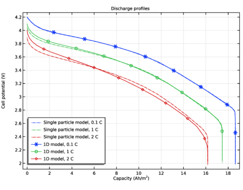
In the associated text field, type Capacity (Ah/m<sup>2</sup>).
7
Select the y-axis label check box.
8
Locate the Legend section. From the Position list, choose Lower left.
Global
1
In the Model Builder window, expand the Cell Potential (spb) node, then click Global.
2
In the Settings window for Global, locate the x-Axis Data section.
3
From the Parameter list, choose Expression.
4
In the Expression text field, type (t[s]/1[h])*i_1C*a.
5
Click to expand the Coloring and Style section. Find the Line style subsection. From the Line list, choose Dash-dot.
6
Click to expand the Legends section. From the Legends list, choose Evaluated.
7
In the Legend text field, type Single particle model, eval(a) C.
8
In the Cell Potential (spb) toolbar, click  Plot.
Table 1
1
In the Results toolbar, click  Table.
2
In the Settings window for Table, locate the Data section.
3
Click Import.
4
Table 2
1
In the Results toolbar, click  Table.
2
In the Settings window for Table, locate the Data section.
3
Click Import.
4
Table 3
1
In the Results toolbar, click  Table.
2
In the Settings window for Table, locate the Data section.
3
Click Import.
4
Table Graph 1
1
In the Model Builder window, right-click Cell Potential (spb) and choose Table Graph.
2
In the Settings window for Table Graph, locate the Coloring and Style section.
3
From the Color list, choose Cycle (reset).
4
Find the Line markers subsection. From the Marker list, choose Cycle.
5
Click to expand the Legends section. Select the Show legends check box.
6
From the Legends list, choose Manual.
7
Table Graph 2
1
Right-click Table Graph 1 and choose Duplicate.
2
In the Settings window for Table Graph, locate the Data section.
3
From the Table list, choose Table 2.
4
Locate the Coloring and Style section. From the Color list, choose Cycle.
5
Locate the Legends section. In the table, enter the following settings:
Table Graph 3
1
Right-click Table Graph 2 and choose Duplicate.
2
In the Settings window for Table Graph, locate the Data section.
3
From the Table list, choose Table 3.
4
Locate the Legends section. In the table, enter the following settings:
5
In the Cell Potential (spb) toolbar, click  Plot.
Single Particle Battery (spb)
Next, perform a charge discharge cycling study for a 1C rate.
1
In the Model Builder window, under Component 1 (comp1) click Single Particle Battery (spb).
2
In the Settings window for Single Particle Battery, locate the Operation Mode section.
3
From the Operation mode list, choose Charge-discharge cycling.
4
In the Idch text field, type Iapplied.
5
In the Vmin text field, type Vmin.
6
Select the Include rest period check box.
7
In the trest,dch text field, type trestdch.
8
In the Ich text field, type -Iapplied.
9
In the Vmax text field, type Vmax.
10
Select the Include rest period check box.
11
In the trest,ch text field, type trestch.
Add Study
1
In the Home toolbar, click  Add Study to open the Add Study window.
2
Go to the Add Study window.
3
Find the Studies subsection. In the Select Study tree, select Preset Studies for Selected Physics Interfaces>Time Dependent with Initialization.
4
Click Add Study in the window toolbar.
5
In the Home toolbar, click  Add Study to close the Add Study window.
Study 2
Step 2: Time Dependent
1
In the Model Builder window, under Study 2 click Step 2: Time Dependent.
2
In the Settings window for Time Dependent, locate the Study Settings section.
3
In the Output times text field, type range(0,10,8000).
4
In the Model Builder window, click Study 2.
5
In the Settings window for Study, locate the Study Settings section.
6
Clear the Generate default plots check box.
7
In the Home toolbar, click  Compute.
Results
Plot the charge discharge cycling potential and compare it with text file data stemming from the original 1D model (Figure 2).
Charge Discharge Cycling Potential
1
In the Home toolbar, click  Add Plot Group and choose 1D Plot Group.
2
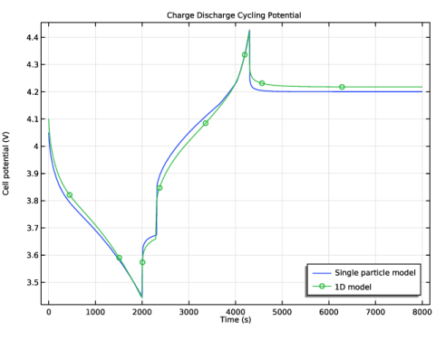
In the Settings window for 1D Plot Group, type Charge Discharge Cycling Potential in the Label text field.
3
Locate the Title section. From the Title type list, choose Label.
4
Locate the Plot Settings section. Select the x-axis label check box.
5
6
Select the y-axis label check box.
7
8
Locate the Legend section. From the Position list, choose Lower right.
9
Locate the Data section. From the Dataset list, choose Study 2/Solution 3 (sol3).
Global 1
1
Right-click Charge Discharge Cycling Potential and choose Global.
2
In the Settings window for Global, click Replace Expression in the upper-right corner of the y-Axis Data section. From the menu, choose Component 1 (comp1)>Single Particle Battery>spb.E_cell - Cell potential - V.
3
Locate the Legends section. From the Legends list, choose Manual.
4
Table 4
1
In the Results toolbar, click  Table.
2
In the Settings window for Table, locate the Data section.
3
Click Import.
4
Table Graph 1
1
In the Model Builder window, right-click Charge Discharge Cycling Potential and choose Table Graph.
2
In the Settings window for Table Graph, locate the Data section.
3
From the Table list, choose Table 4.
4
Locate the Coloring and Style section. Find the Line markers subsection. From the Marker list, choose Circle.
5
Locate the Legends section. Select the Show legends check box.
6
From the Legends list, choose Manual.
7
8
In the Charge Discharge Cycling Potential toolbar, click  Plot.