|
|
|
|
1
|
|
2
|
In the Select Physics tree, select Electrochemistry>Primary and Secondary Current Distribution>Secondary Current Distribution (cd).
|
|
3
|
Click Add.
|
|
4
|
|
5
|
Click Add.
|
|
6
|
|
7
|
Click
|
|
8
|
|
9
|
Click
|
|
1
|
|
2
|
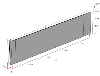
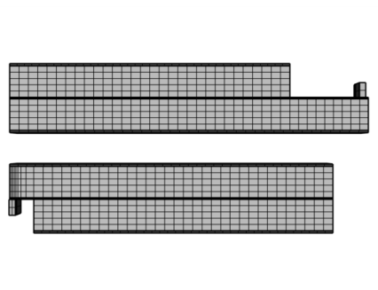
Browse to the model’s Application Libraries folder and double-click the file jelly_roll_flattened_geom_sequence.mph.
|
|
3
|
|
1
|
|
2
|
|
3
|
|
4
|
|
5
|
Click
|
|
6
|
|
7
|
|
1
|
|
2
|
|
1
|
|
2
|
|
3
|
|
4
|
Browse to the model’s Application Libraries folder and double-click the file jelly_roll_flattened_parameters.txt.
|
|
1
|
|
2
|
In the tree, select Built-in>Aluminum.
|
|
3
|
|
4
|
In the tree, select Built-in>Copper.
|
|
5
|
|
6
|
|
7
|
|
8
|
|
9
|
|
10
|
|
11
|
|
12
|
|
1
|
|
2
|
|
1
|
|
2
|
|
3
|
|
1
|
|
2
|
|
3
|
|
1
|
In the Model Builder window, click NMC 111, LiNi0.33Mn0.33Co0.33O2 (Positive, Li-ion Battery) (mat4).
|
|
2
|
|
3
|
|
1
|
|
2
|
|
3
|
|
1
|
|
2
|
|
3
|
|
1
|
In the Model Builder window, under Component 1 (comp1)>Secondary Current Distribution (cd) click Electrolyte 1.
|
|
2
|
|
3
|
|
1
|
|
2
|
|
3
|
|
1
|
|
2
|
|
3
|
|
4
|
Locate the Electrolyte Current Conduction section. From the σl list, choose User defined. In the associated text field, type sigmal_eff.
|
|
5
|
|
6
|
Locate the Electrode Current Conduction section. From the σs list, choose User defined. In the associated text field, type sigmas_eff.
|
|
7
|
|
1
|
|
2
|
|
3
|
|
4
|
|
5
|
|
1
|
|
2
|
|
3
|
|
1
|
|
2
|
|
3
|
|
4
|
|
1
|
|
2
|
|
3
|
|
1
|
|
2
|
|
3
|
|
1
|
|
2
|
|
3
|
|
1
|
|
2
|
|
3
|
|
4
|
|
5
|
|
6
|
|
1
|
In the Model Builder window, under Component 1 (comp1)>Materials click LiPF6 in 3:7 EC:EMC (Liquid, Li-ion Battery) (mat5).
|
|
2
|
|
1
|
|
2
|
|
1
|
|
2
|
|
3
|
|
4
|
|
5
|
|
7
|
|
9
|
|
11
|
|
13
|
|
15
|
|
17
|
|
19
|
|
1
|
|
2
|
|
3
|
|
4
|
|
5
|
|
6
|
|
8
|
|
10
|
|
12
|
|
14
|
|
16
|
|
18
|
|
20
|
|
1
|
|
2
|
In the Settings window for Electrolyte Potential, type Electrolyte Potential Coupling 1 in the Label text field.
|
|
3
|
|
4
|
|
1
|
|
2
|
In the Settings window for Electrolyte Potential, type Electrolyte Potential Coupling 2 in the Label text field.
|
|
3
|
|
4
|
|
1
|
|
2
|
|
3
|
|
4
|
|
1
|
|
2
|
|
3
|
|
4
|
|
5
|
|
6
|
In the Show More Options dialog box, in the tree, select the check box for the node Physics>Advanced Physics Options.
|
|
7
|
Click OK.
|
|
1
|
In the Model Builder window, under Component 1 (comp1)>Secondary Current Distribution (cd) click Continuity 1.
|
|
2
|
|
3
|
|
1
|
|
2
|
|
1
|
|
2
|
|
1
|
|
2
|
|
3
|
|
4
|
|
1
|
|
2
|
|
3
|
|
4
|
|
1
|
|
2
|
|
3
|
|
4
|
|
5
|
|
6
|
|
7
|
In the associated text field, type H_tab_outside_jr/5.
|
|
1
|
|
2
|
|
3
|
Click the Custom button.
|
|
4
|
|
5
|
|
1
|
|
2
|
|
3
|
|
4
|
|
1
|
|
2
|
|
3
|
|
1
|
|
2
|
|
3
|
|
4
|
|
1
|
|
2
|
|
3
|
|
4
|
|
5
|
|
1
|
|
2
|
|
3
|
|
4
|
|
1
|
|
2
|
|
3
|
|
1
|
|
2
|
|
3
|
|
4
|
|
5
|
|
6
|
|
7
|
|
1
|
|
2
|
|
1
|
|
2
|
|
4
|
|
5
|
|
6
|
|
7
|
|
1
|
|
2
|
|
1
|
|
2
|
|
3
|
|
4
|
|
5
|
|
1
|
|
2
|
|
3
|
|
4
|
|
5
|
|
6
|
|
7
|
|
8
|
|
1
|
|
2
|
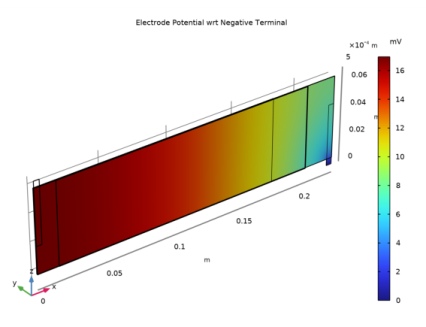
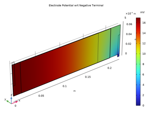
In the Settings window for 3D Plot Group, type Electrode Potential wrt Negative Terminal in the Label text field.
|
|
3
|
|
4
|
|
1
|
|
2
|
In the Settings window for Volume, click Replace Expression in the upper-right corner of the Expression section. From the menu, choose Component 1 (comp1)>Secondary Current Distribution>cd.phis - Electric potential - V.
|
|
3
|
|
4
|
|
1
|
|
2
|
|
3
|
|
4
|
|
1
|
In the Model Builder window, right-click Electrode Potential wrt Negative Terminal and choose Duplicate.
|
|
2
|
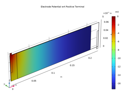
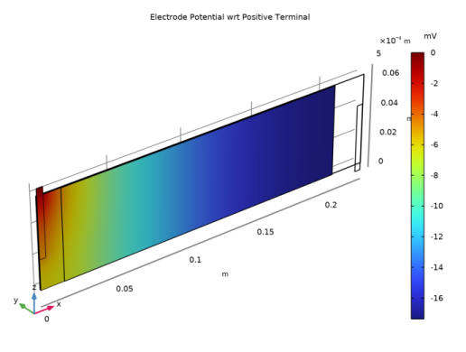
In the Settings window for 3D Plot Group, type Electrode Potential wrt Positive Terminal in the Label text field.
|
|
1
|
In the Model Builder window, expand the Electrode Potential wrt Positive Terminal node, then click Volume 1.
|
|
2
|
In the Settings window for Volume, click Insert Expression (Ctrl+Space) in the upper-right corner of the Expression section. From the menu, choose Component 1 (comp1)>Secondary Current Distribution>cd.phis0_ec1 - Electric potential on boundary - V.
|
|
3
|
|
4
|
|
1
|
|
2
|
|
3
|
|
4
|
|
1
|
|
2
|
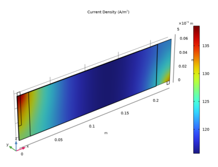
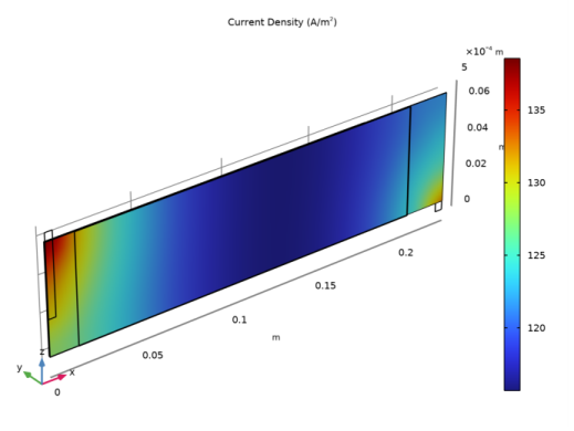
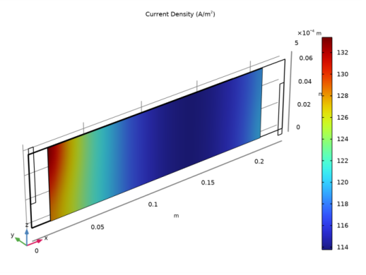
In the Settings window for 3D Plot Group, type Electrolyte Current Density, Separator 1 in the Label text field.
|
|
1
|
|
2
|
In the Settings window for Surface, click Replace Expression in the upper-right corner of the Expression section. From the menu, choose Component 1 (comp1)>Secondary Current Distribution>cd.nIl - Normal electrolyte current density - A/m².
|
|
3
|
|
1
|
|
2
|
|
3
|
|
1
|
|
2
|
|
3
|
|
4
|
|
5
|
|
1
|
|
2
|
|
3
|
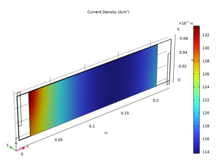
In the Settings window for 3D Plot Group, type Electrolyte Current Density, Separator 2 in the Label text field.
|
|
1
|
In the Model Builder window, expand the Results>Electrolyte Current Density, Separator 2>Surface 1 node, then click Selection 1.
|
|
2
|
|
3
|
|
4
|