Jelly Roll

A lithium battery cell is constructed as a sandwich of different layers (current collector metal foils, porous electrodes, separators), which is placed in an enclosure filled with electrolytes. The configuration of the sandwich depends on the type of enclosure (coin cell, prismatic, pouch, cylinder, and so on). Cylindrical lithium-ion batteries are manufactured by rolling the different battery layers into a cylindrical roll, which is then placed in a metal can. The resulting rolled spiral structure is commonly referred to as a “jelly roll.”

The current collector foils are usually made of copper on the negative side and aluminum on the positive side, with thicknesses around tens of micrometers or less. To conduct the current to and from the jelly roll to the world exterior to the battery can, additional strips of metal are welded to the current collectors. These metal strips are called tabs. The simplest tabbing design, used in low-power batteries, places one tab on each side of the jelly roll (Ref. 1).

The interplay of the various dimensions of the layers and the tabs, in combination with the magnitude of the cell current, governs the temperature and current distribution in the battery cell.

This tutorial models the ohmic and activation losses, and the resulting temperature distribution, in a jelly roll for a pseudostationary case at a constant cell current.

Model Definition

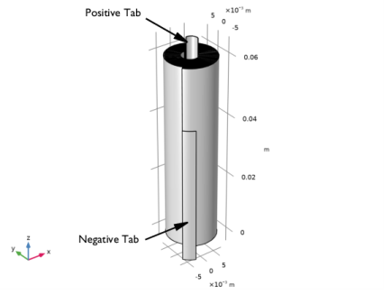
Figure 1 shows the model geometry. The roll is 60 mm high, with a maximum outer spiral radius of 8.5 mm, and a minimum inner radius of 2 mm, including the cell tab. The tabs extend 5 mm outside the jelly roll, the positive upward from the center of the spiral, the negative downward

Figure 1: Model geometry.

Parametric curves, based on archimedal spiral functions are used to create the roll cross-sectional geometry, assuming a constant cell thickness. The following materials and thicknesses are used for the different layers, as indicated in Figure 2:

•

Positive tab: aluminum, 100 mm thick, 4 mm wide

•

Positive current collector: aluminum, 10 mm thick

•

Positive electrode: NMC 111, 200 mm thick

•

Separator: 30 mm thick

•

Negative electrode: graphite, 200 mm thick

•

Negative current collector: copper, 10 mm thick

•

Negative tab: nickel, 100 mm thick, 4 mm wide

Figure 2: Cross section of the jelly roll.

The model in the tutorial uses a pseudostationary approach, only accounting for the ohmic voltage losses in the electronic conductors and the electrolyte and the activation overpotentials due to the charge transfer reactions in the electrodes. The current distribution is modeled using a interface.

This model is a simplification since it will be excluding any (tertiary) effects due to accumulation or depletion of lithium atoms in the electrodes or ions in the electrolyte. As soon as a current starts running through the battery, local concentration levels will change, which in turn impact the local electrolyte conductivity and equilibrium (half-cell) potentials of the electrodes, which will impact the current distribution over time. However, for a short period of time after turning on the current, a secondary current distribution model can accurately predict the voltage losses in the jelly roll.

In the current distribution model, a ground condition is used at the negative terminal, whereas a 1C total current condition is applied at the positive terminal.

The temperature distribution in the jelly roll is modeled using a interface, applying the resulting heat sources from the current distribution model using an multiphysics node. A convective cooling boundary condition on the outer area of the jelly roll is used, prescribing a cooling heat flux being proportional to the surface temperature and the exterior temperature (25°C). Heat being conducted through the electric terminals at the tab ends is ignored.

Results and Discussion

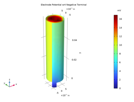
Figure 3 and Figure 4 show the simulated potential distribution in the negative and positive current collectors, respectively, for the jelly roll when subjected to a 1C discharge.

Figure 3: Potential in the negative current collector and tab.

Figure 4: Potential in the positive current collector and tab.

Figure 5 shows a steep increase in temperature in the tabs close to the current terminals. This indicates that the Joule heating in the tabs results in significant local heating already for this fairly small battery at moderate currents. This is important since local temperature differences can result in the battery aging in an inhomogeneous way, which in turn may accelerate aging further.

Figure 5: Temperature distribution.

Notes About the COMSOL Implementation

Assembly boundaries are placed in the middle of the separators, thereby allowing for sweeping the meshes in the through-plane direction.

Reference

1. X. Yao and M. Pecht, “Tab Design and Failures in Cylindrical Li-ion Batteries,” IEEE Access, vol. 7, pp. 24082–24095, 2019.

Battery_Design_Module/Thermal_Management/jelly_roll

Modeling Instructions

This model is built in two parts. In the first part, a secondary current distribution model will be defined and solved. In the second part, heat transfer will included.

From the menu, choose .

New

In the window, click

Model Wizard

In the window, click

In the tree, select .

Click .

Click

In the tree, select .

Click

Geometry 1

Insert a geometry sequence from a file.

In the toolbar, click and choose .

Browse to the model’s Application Libraries folder and double-click the file jelly_roll_geom_sequence.mph.

In the toolbar, click

Global Definitions

Geometry Parameters

By importing the sequence, some parameters were added to the model.

In the window, under click .

In the window for , type Geometry Parameters in the text field.

Physics Parameters

Import additional parameters, needed to set up the physics, as follows:

In the toolbar, click

and choose .

In the window for , type Physics Parameters in the text field.

Locate the section. Click

Browse to the model’s Application Libraries folder and double-click the file jelly_roll_parameters.txt.

Geometry 1

In the window, collapse the node.

Materials

In the toolbar, click

and choose .

Add Material

Go to the window.

In the tree, select .

Right-click and choose .

In the tree, select .

Right-click and choose .

In the tree, select .

Right-click and choose .

In the tree, select .

Right-click and choose .

In the tree, select .

Right-click and choose .

In the toolbar, click

to close the window.

Materials

Aluminum (mat1)

In the window for , locate the section.

From the list, choose .

Copper (mat2)

In the window, click .

In the window for , locate the section.

From the list, choose .

Graphite, LixC6 MCMB (Negative, Li-ion Battery) (mat3)

In the window, click .

In the window for , locate the section.

From the list, choose .

NMC 111, LiNi0.33Mn0.33Co0.33O2 (Positive, Li-ion Battery) (mat4)

In the window, click .

In the window for , locate the section.

From the list, choose .

LiPF6 in 3:7 EC:EMC (Liquid, Li-ion Battery) (mat5)

In the window, click .

In the window for , locate the section.

From the list, choose .

Nickel

The negative tab consists of nickel metal, which is not available in the material library. Add a blank material node for nickel for now. We will add the required parameters later.

In the window, right-click and choose .

In the window for , type Nickel in the text field.

Locate the section. From the list, choose .

Secondary Current Distribution (cd)

Electrolyte 1

Now start defining the current distribution model.

In the window, under click .

In the window for , locate the section.

From the σl list, choose . In the associated text field, type sigmal_eff.

Electrode 1

In the toolbar, click

and choose .

In the window for , locate the section.

From the list, choose .

The electrode node defines electronic conduction in the metal phase domains. The conductivity is taken from the Material nodes by default, so no additional settings are needed here.

Porous Electrode 1

In the toolbar, click

and choose .

The porous electrode node defines the both electronic and ionic conduction in the electrode and electrolyte phases, respectively. Since we use the same settings in the positive and negative electrode materials in this tutorial, it suffices to use one single node.

In the window for , locate the section.

From the list, choose .

Locate the section. From the σl list, choose . In the associated text field, type sigmal_eff.

From the list, choose .

Locate the section. From the σs list, choose . In the associated text field, type sigmas_eff.

From the list, choose .

Porous Electrode Reaction 1

In this tutorial we are only interested in the voltage losses, not the resulting cell voltage. Therefore we use the default value of 0 V for the equilibrium potential in both electrodes. The resulting potential at the positive current terminal will thereby equal the total polarization of the cell.

In the window, click .

In the window for , locate the section.

From the list, choose .

In the i0 text field, type i0.

Locate the section. In the av text field, type Av.

Electric Ground 1

In the toolbar, click

and choose .

In the window for , locate the section.

From the list, choose .

Electrode Current 1

In the toolbar, click

and choose .

In the window for , locate the section.

From the list, choose .

Locate the section. In the Is,total text field, type I_1C.

Materials

Nickel (mat6)

The Nickel material node is now with a small red cross, indicating a missing parameter value.

In the window, under click .

In the window for , locate the section.

In the table, enter the following settings:


Property	Variable	Value	Unit	Property group
Electrical conductivity	sigma_iso ; sigmaii = sigma_iso, sigmaij = 0	1.4e7[S/m]	S/m	Basic

The small red cross should now have disappeared.

Mesh 1

Create a mesh sequence that sweeps the mesh in the radial direction of the spiral. The boundary faces located between the tabs and the current collector foils are meshed first. In this way, these faces will be used as source boundaries by the sweep operation, and the mid-separator boundaries will be used as destination boundaries. As prerequisite for sweeping the mesh is that, by the way the geometry sequence is set up, assembly boundaries are located in the middle of the separators. Using a geometry without an assembly would not allow for sweeping, since it would introduce faces on the destination boundaries that would not correspond to any faces on the source boundaries.

Size 1

In the window, under right-click and choose .

In the window for , locate the section.

From the list, choose .

Locate the section. Click the button.

Locate the section. Select the check box.

In the associated text field, type H_tab_outside_jr/5.

Size

In the window, click .

In the window for , locate the section.

Click the button.

Locate the section. In the text field, type H_mesh.

In the text field, type D_sep/2.

Free Quad 1

In the toolbar, click

and choose .

In the window for , locate the section.

From the list, choose .

Click

Swept 1

In the toolbar, click

Distribution 1

Right-click and choose .

In the window for , locate the section.

From the list, choose .

Locate the section. In the text field, type 2.

Distribution 2

In the window, right-click and choose .

In the window for , locate the section.

From the list, choose .

Distribution 3

Right-click and choose .

In the window for , locate the section.

From the list, choose .

Locate the section. In the text field, type 2.

Swept 1

Right-click and choose .

Study 1

Now solve the current distribution model.

In the window, click .

In the window for , locate the section.

Clear the check box.

In the toolbar, click

Results

Add plots for the potentials as follows:

Electrode Potential wrt Negative Terminal

In the toolbar, click

and choose .

In the window for , type Electrode Potential wrt Negative Terminal in the text field.

Volume 1

Right-click and choose .

In the window for , click in the upper-right corner of the section. From the menu, choose .

Locate the section. From the list, choose .

Selection 1

Right-click and choose .

In the window for , locate the section.

From the list, choose .

Electrode Potential wrt Negative Terminal

In the window, under click .

In the window for , click to expand the section.

From the list, choose .

Locate the section. Select the check box.

Locate the section. Clear the check box.

In the toolbar, click

Electrode Potential wrt Positive Terminal

Right-click and choose .

In the window for , type Electrode Potential wrt Positive Terminal in the text field.

Volume 1

In the window, expand the node, then click .

In the window for , click in the upper-right corner of the section. From the menu, choose .

Locate the section. In the text field, type cd.phis-cd.phis0_ec1.

From the list, choose .

Selection 1

In the window, expand the node, then click .

In the window for , locate the section.

From the list, choose .

Electrode Potential wrt Positive Terminal

In the window, under click .

In the toolbar, click

Component 1 (comp1)

Now we move over to the second part of this tutorial, in which we will include heat transfer.

In the toolbar, click

and choose .

Add Physics

Go to the window.

In the tree, select .

Click in the window toolbar.

In the toolbar, click

to close the window.

Heat Transfer in Solids (ht)

Solid 1

The default node will define heat transfer in all domains. The thermal conductivity is taken from the materials nodes by default. Since we will defining a stationary problem, the density and the heat capacity are not needed.