PDF

Pressure Reciprocity Calibration Coupler with Detailed Moist Air Material Properties
Introduction
When high-fidelity measurement microphones are calibrated, a pressure reciprocity calibration method is used. During calibration, two microphones are connected at each end of a closed cylindrical cavity. For the calibration procedure, it is important to understand the acoustic field inside such a cavity, including all the thermoviscous acoustic effects, for example, the acoustic boundary layers at higher frequencies and the transition to isothermal behavior at the lower frequencies.
This model sets up a simple calibration coupler model and discusses important considerations when performing a high-precision absolute-value simulation. The model results include the acoustic transfer impedance used for reciprocity calibration and the pressure in the coupler. The results are compared with analytical predictions.
The model also includes precise material property estimation using the Thermodynamics functionality in COMSOL Multiphysics. This allows setting up a moist air material that depends on the ambient pressure, temperature, and relative humidity. This functionality is available with the Liquid & Gas Properties Module. The model can also be set up using the default air material found in the Material Library, but this will represent dry air.
Figure 1: Sketch of a typical pressure reciprocity calibration coupler with two microphones. The cylindrical rz-coordinate system used in the model is also indicated, as well as the source and receiver boundaries.
Model Definition
In order to calibrate microphones a commonly used technique is the reciprocity calibration approach. The method relies on using microphones both as source and receivers (they are reciprocal) in a well described coupled setup (see Ref. 1 and 2). The setup consisting of two microphones and a coupler volume, is sketched in Figure 1. The coupler has a length L and a radius a. Both are parameters that can be changed in the COMSOL model to fit the dimensions of various standardized couplers. A 2D axisymmetric representation is used on the COMSOL model.
The ratio between the input current Iin and the output voltage Vout is the electric transfer impedance Ze (this quantity is measured). The acoustic transfer impedance Za of the coupler is the ratio between the average pressure at the receiver boundary pav,r and the volume velocity at the source boundary Qs. The product of the microphone sensitivity M of microphone A and microphone B is given as
Using three microphones (A, B, and C), in all combinations of source and receiver, results in a system of three equations with the three sensitivities as unknowns. This system is solved to produce the calibrated microphone sensitivities MA, MB, and MC. In this procedure, it is assumed that the acoustic transfer impedance Za of the coupler volume is known. To achieve high precision calibration the acoustic transfer impedance has to be well defined for a large frequency. Material properties of air also need to be well described.
The calibration procedure, acoustic transfer impedance, and material properties are described by the international standard, IEC 61094-2:2009, Ref. 3. As an alternative to the IEC standard, you can choose to model the acoustic transfer impedance in full detail using the Thermoviscous Acoustics, Frequency Domain physics interface. Detailed moist air material properties can be computed using the Thermodynamics feature. This will yield an acoustic transfer impedance that is correct at all frequencies. The simulation only assumes linear acoustics, while modeling all thermoviscous effects in details. That is, the dynamics of the thermal and viscous boundary layers, as well as the complex transition from adiabatic to isothermal behavior for decreasing frequencies. In the limit of large couplers and high frequencies correct wave propagation behavior is also captured.
The acoustic transfer impedance is computed in this model and compared to three different analytical models, as described below.
Isothermal Limit, Very Low Frequency
At very low frequencies the system behaves isothermally (the thermal boundary layers fill the entire coupler volume). The pressure change dp, in the volume V, for a given volume change dV, follows from the definition of isothermal compressibility
The variables for this expression are located under Definitions > Variables - Isothermal Limit (very low frequency).
Transmission Line, High Frequency
In the high frequency limit, disregarding boundary layer effects on the source and receiver boundaries, the coupler can be approximated with a transmission line defined by a transfer matrix T. The model takes the boundary layer losses at the coupler walls into account through a complex-valued characteristic specific impedance and propagation constant. Details and an expression for the transfer matrix is described in the tutorial Wax Guard Acoustics: Transfer Matrix Computation. The acoustic transfer impedance (when the receiver is sound hard) is the simply defined as Za = 1/T21. and the admittance is directly given by T21.
The variables for this analytical model are located under Definitions > Transmission Line (high frequency).
Model by Vincent et al., Low Frequency
More advanced analytical models exist for computing the transfer impedance of a cylinder, including all viscous and thermal effects. In a recent work by Vincent and others (see Ref. 5), the work of Gerber (see Ref. 4) is extended to be valid in the full low frequency range (from medium all the way to very low frequencies and the isothermal limit). The pressure in the coupler and the transfer impedance are given by equations 24, 26, 27, and 30 in Ref. 5. Note that the source and receiver admittances are 0 (perfect source and sound hard wall).
One of the analytical expressions include an infinite sum. In COMSOL, the sum is implemented using the sum() operator, with 10 terms in the sum. The analytical model also includes zeros of the Bessel function, the first 10 used are tabulated in the interpolation function lam_n() defined under Definitions.
The variables for this analytical model are located under Definitions>Vincent et al. (low frequency).
Results and Discussion
The root mean square (RMS) velocity in the coupler and the temperature fluctuations, for four evaluation frequencies of 0.1 Hz, 1 Hz, 10 Hz, and 100 Hz, is depicted in Figure 2 and Figure 3, respectively. The dependency of the viscous and thermal boundary layers on frequency and the extent into the geometry, can be seen graphically. In the model, the coupler has a length L of 5 mm and a radius a of 4.5 mm.
The real and imaginary part of the pressure in the coupler is depicted in Figure 4 and Figure 5, respectively. The graphs show the expected correlation between the COMSOL model and the analytical models. The isothermal limit represents the asymptotic behavior for the frequency going to 0. The transmission line model shows the best agreement on the high frequency limit, without giving a perfect match. The model by Vincent and others agrees well with the COMSOL model (within 0.01 dB) on the real part below about 150 Hz and for the imaginary part below about 5 Hz.
The real and imaginary part of the acoustic transfer impedance Za, is plotted as function of frequency in Figure 6. The graph again shows good correlation between the model by Vincent et al. for frequencies below 100 Hz. Having consistent and correct values of the acoustic transfer impedance is essential for high fidelity calibration.
In this tutorial, the moist air material generated using the Predefined System option for Moist air of the Thermodynamics feature is used. This functionality requires the Liquid & Gas Properties Module. Once the mixture is set up using the steps of the wizard a moist air material is generated using the Generate Material option. Note that the content of the various species (mole fractions) that make up air, can be modified in the Local properties table inside the Materials > Gas: Moist Air 1 material. This allows to model any air variant.
As an example, the dependency on the ambient temperature of the density, the dynamic viscosity, the thermal conductivity, and the speed of sound is depicted in Figure 7. The graphs shows the values for four values of the relative humidity. This dependency is automatically included in the COMSOL model results as Relative humidity φw, is a Model Input when the moist air material is used.
Figure 2: Acoustic velocity fluctuations (RMS) in the coupler volume at 0.1, 1, 10, and 100 Hz.
Figure 3: Acoustic temperature fluctuations in the coupler at 0.1, 1, 10, and 100 Hz.
Figure 4: Real part of the pressure in the coupler evaluated using the COMSOL model and the three analytical approximations.
Figure 5: Imaginary part of the pressure in the coupler evaluated using the COMSOL model and the three analytical approximations.
Figure 6: Acoustic transfer impedance for the coupler volume evaluated using the COMSOL model as well as the low and high frequency models.
Figure 7: Various material properties of moist air (density, dynamic viscosity, thermal conductivity, and speed of sound) evaluated as function of temperature (from 0 to 50 deg C) for four different values of the relative humidity (0.0, 0.2, 0.4, and 0.8).
Notes About the COMSOL Implementation
Bulk Losses
When modeling fluids with the thermoviscous acoustics interface, the damping and dissipation due to the thermal and viscous boundary layers is included in full detail. In the bulk/volume of the fluid (away from the boundaries) the model captures the attenuation that corresponds to the classical thermoviscous attenuation αtv. This is not the correct bulk attenuation as it does not include losses due to relaxation. These losses that are, for example, captured when using the Atmosphere attenuation model in pressure acoustics. In most microacoustic applications the boundary layer losses are orders of magnitude higher than the bulk losses, so it is not important. In the present coupler application, the bulk losses may start to play a small role at very high frequencies. In this case, the true bulk losses may be included by defining a frequency dependent bulk viscosity μB = μB(f), according to
where ω = 2πf and α is the true atmosphere attenuation. This will introduce consistent bulk/volume losses that also include relaxation processes and other mechanisms included in the expression for α.
Membrane Deformation
In this model, plane wave propagation is assumed. For certain larger couplers, the effects of the true membrane deformation can start to play a role a high frequencies. In this case, the membrane can be included in the model. See for example The Brüel & Kjær 4134 Condenser Microphone tutorial.
Mesh
The mesh used in this model uses two boundary layer meshes. The first resolves the physics by resolving the thermal and viscous boundary layer thickness (also known as the penetration depth). The second adds a small single layer that is used to resolve the numerical singularities at the corners of the geometry.
References
1. Danish Primary Laboratory of Acoustic Microphone Reciprocity Calibration Calculation Program for Reciprocity Calibration, Technical Review No. 1-1998, Brüel & Kjær, Denmark.
2. E. Frederiksen, “Acoustic metrology - an overview of calibration methods and their uncertainty,” Int. J. Metrol. Qual. Eng., vol. 4, pp. 97–107, 2013.
3. International Standard, Electroacoustics - Measurement microphones - Part 2: Primary method for pressure calibration of laboratory standard microphones by the reciprocity technique, IEC 61094-2:2009.
4. H. Gerber, “Acoustic Properties of Flui.Filled Chambers at Infrasonic Frequencies in the Absence of Convection,” J. Acoust. Soc. Am., vol. 36, p. 1427, 1964.
5. P. Vincent, D. Rodrigues, F. Larsonnier, C. Guianvarc’h, and S. Durand, “Acoustic transfer admittance of cylindrical cavities in infrasonic frequency range,” Meterologica, vol. 56, p. 015003, 2019.
Application Library path: Acoustics_Module/Tutorials,_Thermoviscous_Acoustics/pressure_reciprocity_calibration_coupler
Modeling Instructions
From the File menu, choose New.
New
In the New window, click  Model Wizard.
Model Wizard
1
In the Model Wizard window, click  2D Axisymmetric.
2
In the Select Physics tree, select Acoustics>Thermoviscous Acoustics>Thermoviscous Acoustics, Frequency Domain (ta).
3
Click Add.
4
Click  Study.
5
In the Select Study tree, select General Studies>Frequency Domain.
6
Global Definitions
Parameters - Physics
1
In the Model Builder window, under Global Definitions click Parameters 1.
2
In the Settings window for Parameters, type Parameters - Physics in the Label text field.
3
Locate the Parameters section. Click  Load from File.
4
Browse to the model’s Application Libraries folder and double-click the file pressure_reciprocity_calibration_coupler_parameters_physics.txt.
Parameters - Geometry
1
In the Home toolbar, click  Parameters and choose Add>Parameters.
2
In the Settings window for Parameters, type Parameters - Geometry in the Label text field.
3
Locate the Parameters section. Click  Load from File.
4
Browse to the model’s Application Libraries folder and double-click the file pressure_reciprocity_calibration_coupler_parameters_geometry.txt.
Geometry 1
Rectangle 1 (r1)
1
In the Geometry toolbar, click  Rectangle.
2
In the Settings window for Rectangle, locate the Size and Shape section.
3
In the Width text field, type a.
4
In the Height text field, type L.
5
Click  Build All Objects.
Add Material
1
In the Home toolbar, click  Add Material to open the Add Material window.
2
Go to the Add Material window.
3
4
Click Add to Component in the window toolbar.
5
In the Home toolbar, click  Add Material to close the Add Material window.
Materials
Air (dry)
1
In the Settings window for Material, type Air (dry) in the Label text field.
You just added the default air material from the Material Library. This is a model of dry air where certain properties like density and speed of sound are based on the ideal gas law. A detailed moist air material can be conveniently set up using a Predefined System defined by the Thermodynamics feature.
Setting up the moist air material requires the Liquid and Gas Properties Module. If you do not have that product, you can skip the next steps and use the Air (dry) material instead.
Global Definitions
In the Physics toolbar, click  Thermodynamics and choose Predefined System.
Select System
1
Go to the Select System window.
2
From the Predefined thermodynamic system list, choose Moist air.
3
Click Next in the window toolbar.
Select Species
1
Go to the Select Species window.
2
Click Next in the window toolbar.
Select Thermodynamic Model
1
Go to the Select Thermodynamic Model window.
2
From the Gas phase model list, choose Peng-Robinson.
The choice of Gas phase model depends on the exterior conditions like ambient pressure and temperature. The different models are described in the Liquid and Gas Properties Module User’s Guide in the Thermodynamics Models section.
3
Click Finish in the window toolbar.
Global Definitions
Moist Air 1 (pp1)
In the Model Builder window, under Global Definitions>Thermodynamics right-click Moist Air 1 (pp1) and choose Generate Material.
Select Species
1
Go to the Select Species window.
2
Click Next in the window toolbar.
Select Properties
1
Go to the Select Properties window.
2
Click Next in the window toolbar.
Define Material
1
Go to the Define Material window.
2
Click Finish in the window toolbar.
Note that the bulk viscosity is defined in terms of the dynamic viscosity. The relation is the same as in the default (dry) air material. Values of the bulk viscosity are experimentally obtained using high-frequency absorption techniques. More details can be found in the Acoustic Properties of Fluids chapter of the Acoustics Module User’s Guide.
Use the moist air material for the model.
Materials
Gas: Moist Air 1 (pp1mat1)
1
In the Model Builder window, under Component 1 (comp1)>Materials click Gas: Moist Air 1 (pp1mat1).
2
Definitions
Variables - Material Properties
1
In the Model Builder window, expand the Component 1 (comp1)>Definitions node.
2
Right-click Definitions and choose Variables.
3
In the Settings window for Variables, type Variables - Material Properties in the Label text field.
4
Locate the Variables section. Click  Load from File.
5
Browse to the model’s Application Libraries folder and double-click the file pressure_reciprocity_calibration_coupler_variables_material.txt.
Variables - Isotermal Limit (very low frequency)
1
Right-click Definitions and choose Variables.
2
In the Settings window for Variables, type Variables - Isotermal Limit (very low frequency) in the Label text field.
3
Locate the Variables section. Click  Load from File.
4
Browse to the model’s Application Libraries folder and double-click the file pressure_reciprocity_calibration_coupler_variables_isothermal.txt.
Variables - Transmission Line (high frequency)
1
Right-click Definitions and choose Variables.
2
In the Settings window for Variables, type Variables - Transmission Line (high frequency) in the Label text field.
3
Locate the Variables section. Click  Load from File.
4
Browse to the model’s Application Libraries folder and double-click the file pressure_reciprocity_calibration_coupler_variables_transmission.txt.
Variables - Vincent et al. (low frequency)
1
Right-click Definitions and choose Variables.
2
In the Settings window for Variables, type Variables - Vincent et al. (low frequency) in the Label text field.
3
Locate the Variables section. Click  Load from File.
4
Browse to the model’s Application Libraries folder and double-click the file pressure_reciprocity_calibration_coupler_variables_vincent.txt.
Integration 1 (intop1)
1
In the Definitions toolbar, click  Nonlocal Couplings and choose Integration.
2
In the Settings window for Integration, type intop_s in the Operator name text field.
3
Locate the Source Selection section. From the Geometric entity level list, choose Boundary.
4
Integration 2 (intop2)
1
In the Definitions toolbar, click  Nonlocal Couplings and choose Integration.
2
In the Settings window for Integration, type intop_r in the Operator name text field.
3
Locate the Source Selection section. From the Geometric entity level list, choose Boundary.
4
Integration 3 (intop3)
1
In the Definitions toolbar, click  Nonlocal Couplings and choose Integration.
2
In the Settings window for Integration, type intop_pnt in the Operator name text field.
3
Locate the Source Selection section. From the Geometric entity level list, choose Point.
4
5
Locate the Advanced section. Clear the Compute integral in revolved geometry check box.
Interpolation 1 (int1)
1
In the Definitions toolbar, click  Interpolation.
2
In the Settings window for Interpolation, locate the Definition section.
3
From the Data source list, choose File.
4
Click  Browse.
5
Browse to the model’s Application Libraries folder and double-click the file pressure_reciprocity_calibration_coupler_bessel_zeros.txt.
6
Click  Import.
7
In the Function name text field, type lam_n.
8
Locate the Interpolation and Extrapolation section. From the Interpolation list, choose Nearest neighbor.
9
Locate the Units section. In the Argument table, enter the following settings:
10
In the Function table, enter the following settings:
11
Click the  Show More Options button in the Model Builder toolbar.
12
In the Show More Options dialog box, in the tree, select the check box for the node Physics>Advanced Physics Options.
13
Thermoviscous Acoustics, Frequency Domain (ta)
Thermoviscous Acoustics Model 1
1
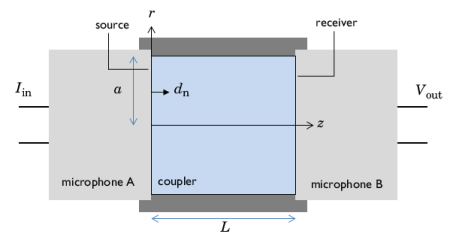
In the Model Builder window, under Component 1 (comp1)>Thermoviscous Acoustics, Frequency Domain (ta) click Thermoviscous Acoustics Model 1.
2
In the Settings window for Thermoviscous Acoustics Model, locate the Model Input section.
3
In the φw text field, type relH.
Because the relative humidity is set up as a Model Input for the moist air material, it automatically appears as an input in the physics.
Velocity 1
1
In the Physics toolbar, click  Boundaries and choose Velocity.
2
3
In the Settings window for Velocity, locate the Velocity section.
4
Select the Prescribed in r direction check box.
5
Select the Prescribed in z direction check box.
6
In the u0z text field, type ta.iomega*dn.
7
Click to expand the Excluded Points section. Select Point 3 only.
Isothermal 1
1
In the Physics toolbar, click  Boundaries and choose Isothermal.
2
In this model, the mesh is set up manually. Proceed by directly adding the desired mesh component.
Mesh 1
Free Triangular 1
In the Mesh toolbar, click  Free Triangular.
Size
1
In the Model Builder window, click Size.
2
In the Settings window for Size, locate the Element Size section.
3
Click the Custom button.
4
Locate the Element Size Parameters section. In the Maximum element size text field, type a/10.
5
In the Minimum element size text field, type dvisc0.
Size 1
1
In the Model Builder window, right-click Free Triangular 1 and choose Size.
2
In the Settings window for Size, locate the Geometric Entity Selection section.
3
From the Geometric entity level list, choose Boundary.
4
5
Locate the Element Size section. Click the Custom button.
6
Locate the Element Size Parameters section. Select the Maximum element size check box.
7
Boundary Layers 1
1
In the Mesh toolbar, click  Boundary Layers.
2
In the Settings window for Boundary Layers, click to expand the Transition section.
3
Clear the Smooth transition to interior mesh check box.
Boundary Layer Properties
1
In the Model Builder window, click Boundary Layer Properties.
2
3
In the Settings window for Boundary Layer Properties, locate the Layers section.
4
From the Thickness specification list, choose First layer.
5
In the Thickness text field, type 0.2*dvisc.
Boundary Layers 2
1
In the Mesh toolbar, click  Boundary Layers.
2
In the Settings window for Boundary Layers, locate the Transition section.
3
Clear the Smooth transition to interior mesh check box.
Boundary Layer Properties
1
In the Model Builder window, click Boundary Layer Properties.
2
3
In the Settings window for Boundary Layer Properties, locate the Layers section.
4
From the Thickness specification list, choose First layer.
5
In the Thickness text field, type 0.2*dvisc.
Boundary Layers 3
1
In the Mesh toolbar, click  Boundary Layers.
2
In the Settings window for Boundary Layers, locate the Transition section.
3
Clear the Smooth transition to interior mesh check box.
Boundary Layer Properties
1
In the Model Builder window, click Boundary Layer Properties.
2
3
In the Settings window for Boundary Layer Properties, locate the Layers section.
4
In the Number of layers text field, type 1.
5
From the Thickness specification list, choose First layer.
6
In the Thickness text field, type 2e-6.
Boundary Layers 4
1
In the Mesh toolbar, click  Boundary Layers.
2
In the Settings window for Boundary Layers, locate the Transition section.
3
Clear the Smooth transition to interior mesh check box.
Boundary Layer Properties
1
In the Model Builder window, click Boundary Layer Properties.
2
3
In the Settings window for Boundary Layer Properties, locate the Layers section.
4
In the Number of layers text field, type 1.
5
From the Thickness specification list, choose First layer.
6
In the Thickness text field, type 2e-6.
7
Click  Build All.
Study 1
Step 1: Frequency Domain
1
In the Model Builder window, under Study 1 click Step 1: Frequency Domain.
2
In the Settings window for Frequency Domain, locate the Study Settings section.
3
Click  Range.
4
In the Range dialog box, choose ISO preferred frequencies from the Entry method list.
5
In the Start frequency text field, type 0.05.
6
In the Stop frequency text field, type 10000.
7
From the Interval list, choose 1/3 octave.
8
Click Replace.
9
In the Home toolbar, click  Compute.
Results
Acoustic Pressure (ta)
RMS Acoustic Velocity (ta)
1
In the Model Builder window, under Results click Acoustic Velocity (ta).
2
In the Settings window for 2D Plot Group, type RMS Acoustic Velocity (ta) in the Label text field.
Surface
1
In the Model Builder window, expand the RMS Acoustic Velocity (ta) node, then click Surface.
2
In the Settings window for Surface, locate the Expression section.
3
In the Expression text field, type ta.v_rms.
4
In the RMS Acoustic Velocity (ta) toolbar, click  Plot.
Temperature Variation (ta)
Pressure in Coupler: real(p)
1
In the Home toolbar, click  Add Plot Group and choose 1D Plot Group.
2
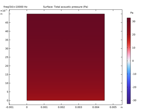
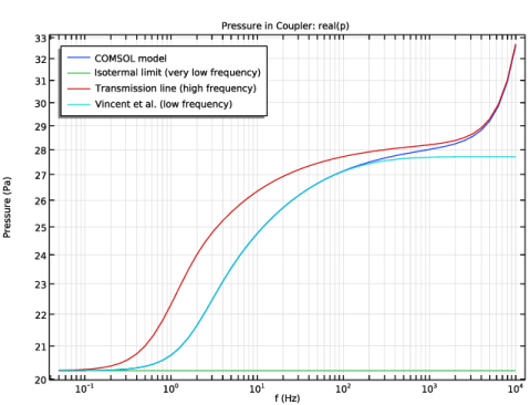
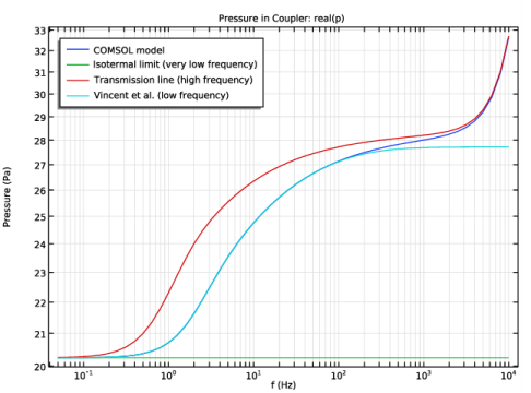
In the Settings window for 1D Plot Group, type Pressure in Coupler: real(p) in the Label text field.
3
Click to expand the Title section. From the Title type list, choose Label.
4
Locate the Plot Settings section. Select the x-axis label check box.
5
6
Select the y-axis label check box.
7
8
Locate the Legend section. From the Position list, choose Upper left.
Point Graph 1
1
Right-click Pressure in Coupler: real(p) and choose Point Graph.
2
3
In the Settings window for Point Graph, locate the y-Axis Data section.
4
In the Expression text field, type real(ta.p_t).
5
Click to expand the Legends section. Select the Show legends check box.
6
From the Legends list, choose Manual.
7
Global 1
1
In the Model Builder window, right-click Pressure in Coupler: real(p) and choose Global.
2
In the Settings window for Global, locate the y-Axis Data section.
3
4
In the Pressure in Coupler: real(p) toolbar, click  Plot.
5
Click the  x-Axis Log Scale button in the Graphics toolbar.
6
Click the  y-Axis Log Scale button in the Graphics toolbar.
Pressure in Coupler: imag(p)
1
Right-click Pressure in Coupler: real(p) and choose Duplicate.
2
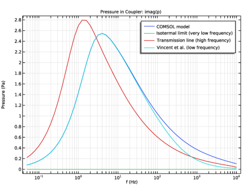
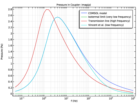
In the Settings window for 1D Plot Group, type Pressure in Coupler: imag(p) in the Label text field.
3
Locate the Legend section. From the Position list, choose Upper right.
Point Graph 1
1
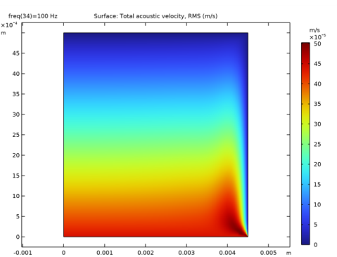
In the Model Builder window, expand the Pressure in Coupler: imag(p) node, then click Point Graph 1.
2
In the Settings window for Point Graph, locate the y-Axis Data section.
3
In the Expression text field, type imag(ta.p_t).
Global 1
1
In the Model Builder window, click Global 1.
2
In the Settings window for Global, locate the y-Axis Data section.
3
4
In the Pressure in Coupler: imag(p) toolbar, click  Plot.
5
Click the  y-Axis Log Scale button in the Graphics toolbar.
Acoustic Transfer Impedance: real(Z) and imag(Z)
1
In the Home toolbar, click  Add Plot Group and choose 1D Plot Group.
2
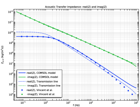
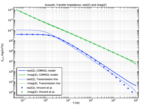
In the Settings window for 1D Plot Group, type Acoustic Transfer Impedance: real(Z) and imag(Z) in the Label text field.
3
Locate the Title section. From the Title type list, choose Label.
4
Locate the Plot Settings section. Select the x-axis label check box.
5
6
Select the y-axis label check box.
7
In the associated text field, type Z<sub>a,12</sub> (kg/(m<sup>4</sup>s)).
8
Locate the Axis section. Select the x-axis log scale check box.
9
Select the y-axis log scale check box.
10
Locate the Legend section. From the Position list, choose Lower left.
Global 1
1
Right-click Acoustic Transfer Impedance: real(Z) and imag(Z) and choose Global.
2
In the Settings window for Global, locate the y-Axis Data section.
3
4
Click to expand the Coloring and Style section. In the Width text field, type 2.
Global 2
1
In the Model Builder window, right-click Acoustic Transfer Impedance: real(Z) and imag(Z) and choose Global.
2
In the Settings window for Global, locate the y-Axis Data section.
3
4
Locate the Coloring and Style section. Find the Line style subsection. From the Line list, choose Dashed.
5
From the Color list, choose Cycle (reset).
Global 3
1
Right-click Acoustic Transfer Impedance: real(Z) and imag(Z) and choose Global.
2
In the Settings window for Global, locate the y-Axis Data section.
3
4
Locate the Coloring and Style section. Find the Line style subsection. From the Line list, choose None.
5
From the Color list, choose Cycle (reset).
6
Find the Line markers subsection. From the Marker list, choose Point.
7
In the Number text field, type 25.
8
In the Acoustic Transfer Impedance: real(Z) and imag(Z) toolbar, click  Plot.
Next create a grid dataset that will be used to plot the material properties as function of temperature for several values of the relative humidity.
Grid 1D 1
1
In the Results toolbar, click  More Datasets and choose Grid>Grid 1D.
2
In the Settings window for Grid 1D, locate the Parameter Bounds section.
3
In the Name text field, type Tg.
4
In the Minimum text field, type 273.15.
5
In the Maximum text field, type 323.15.
Density
1
In the Results toolbar, click  1D Plot Group.
2
In the Settings window for 1D Plot Group, type Density in the Label text field.
3
Locate the Data section. From the Dataset list, choose Grid 1D 1.
4
From the Parameter selection (freq) list, choose First.
5
Locate the Title section. From the Title type list, choose Label.
6
Locate the Plot Settings section. Select the x-axis label check box.
7
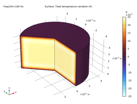
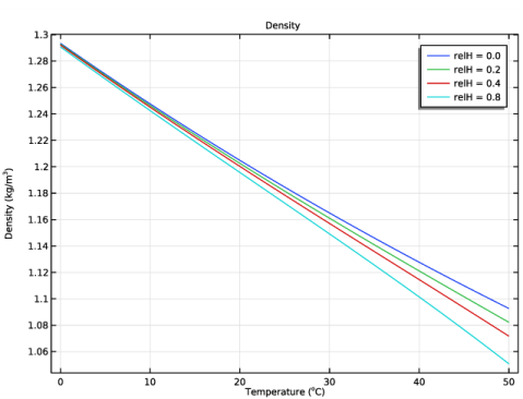
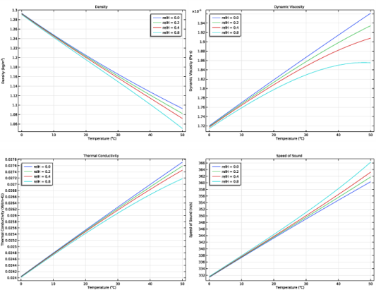
In the associated text field, type Temperature (<sup>o</sup>C).
8
Select the y-axis label check box.
9
In the associated text field, type Density (kg/m<sup>3</sup>).
Line Graph 1
1
Right-click Density and choose Line Graph.
2
In the Settings window for Line Graph, locate the y-Axis Data section.
3
In the Expression text field, type subst(pp1mat1.def.rho,minput.T,Tg[K/m],minput.pA,p0,minput.phi,0).
4
Click to expand the Legends section. Select the Show legends check box.
5
From the Legends list, choose Manual.
6
7
In the Density toolbar, click  Plot.
Line Graph 2
1
Right-click Line Graph 1 and choose Duplicate.
2
In the Settings window for Line Graph, locate the y-Axis Data section.
3
In the Expression text field, type subst(pp1mat1.def.rho,minput.T,Tg[K/m],minput.pA,p0,minput.phi,0.2).
4
Locate the Legends section. In the table, enter the following settings:
5
In the Density toolbar, click  Plot.
Line Graph 3
1
Right-click Line Graph 2 and choose Duplicate.
2
In the Settings window for Line Graph, locate the y-Axis Data section.
3
In the Expression text field, type subst(pp1mat1.def.rho,minput.T,Tg[K/m],minput.pA,p0,minput.phi,0.4).
4
Locate the Legends section. In the table, enter the following settings:
5
In the Density toolbar, click  Plot.
Line Graph 4
1
Right-click Line Graph 3 and choose Duplicate.
2
In the Settings window for Line Graph, locate the y-Axis Data section.
3
In the Expression text field, type subst(pp1mat1.def.rho,minput.T,Tg[K/m],minput.pA,p0,minput.phi,0.8).
4
Locate the Legends section. In the table, enter the following settings:
5
In the Density toolbar, click  Plot.
Duplicate the density plot in order to create plots of the dynamic viscosity (pp1mat1.def.mu), thermal conductivity (pp1mat1.def.k_iso), and speed of sound (pp1mat1.def.c). Finally, group the plots in a Node Group. All the plots are depicted in the Results and Discussion section of the documentation.