This phase transformation model is based on the work of Leblond and Devaux (Ref. 1). The model primarily considers carbon-diffusion-based phase transformations that occur in steels during heat treatment. Such transformations include austenite to ferrite, and austenite to bainite. There are three formulations for the Leblond–Devaux model:

where the phase transformation is active only when ; that is, when the right-hand side of Equation 3-2 is strictly positive. In general, the functions and are functions of temperature T. It was shown in Ref. 1 that the bainitic transformation additionally depends on the rate of cooling, . In this case, the functions and are functions of both T and .

where the phase transformation is active only when ; that is, when the right side of Equation 3-3 is strictly positive. The equilibrium phase fraction and the time constant are typically functions of temperature.

This enables straightforward calibration of the model parameters from TTT diagram data. At a given temperature, the equilibrium phase fraction of the destination phase is . A relative phase fraction of the destination phase is defined such that it is 1.0 as the equilibrium phase fraction is reached. The relative phase fraction X is given by

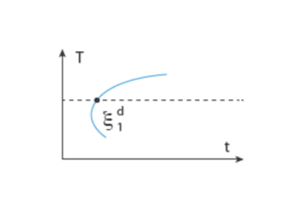
In the TTT diagram in Figure 3-1, a curve representing a fixed destination phase fraction is shown. At a fixed temperature T, this destination phase fraction is reached at time t1, so that

where t1 will vary with temperature, and the relative phase fraction X1 is understood to be the relative phase fraction corresponding to .

This phase transformation model is based on the work by Leblond and others (Ref. 3).

The equilibrium phase fraction , the time constant and the Avrami exponent are typically functions of temperature. On rate form, Equation 3-8 can be expressed as

where the explicit time dependence has been eliminated. The phase transformation is active only when ; that is, when the right side of Equation 3-9 is strictly positive. For the special case of , the equation reduces to the time-and-equilibrium form of the Leblond–Devaux model (Equation 3-3). The JMAK phase transformation model in Equation 3-9 has a mathematical disadvantage in that an initial destination phase fraction equal to zero will yield a trivial zero solution, as the logarithm will evaluate to zero. There are different ways to circumvent this problem. One way is to require the initial phase fraction be assigned a small, but finite, value. Another way is to modify the rate equation itself, so that a zero initial phase fraction does not yield a trivial zero solution. In the phase transformation interfaces, the JMAK phase transformation model in Equation 3-9 is modified for small values on the phase fraction . Below a certain threshold, the argument for the logarithm is modified so that the logarithm does not produce a zero value. This threshold phase fraction is set to 10-6 by default.

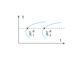
As in the case of the Leblond–Devuax model, the JMAK model can be calibrated using TTT diagram data. The integrated form in Equation 3-8 is used to calibrate the time constant and the Avrami exponent . To calibrate these two phase transformation model parameters, two curves are needed from a TTT diagram, see Figure 3-2. At a fixed temperature T, the two destination phase fractions are reached at times t1 and t2, respectively, so that

where the relative phase fractions X1 and X2 are understood to be the relative phase fractions corresponding to and , respectively. The transformation times t1 and t2 will vary with temperature.

This phase transformation model is based on the work by Kirkaldy and Venugopalan (Ref. 10), and extended and modified by several others. There are two formulations for the Kirkaldy–Venugopalan phase transformation model:

where is the equilibrium phase fraction, is a reference rate that in principle depends on temperature, chemical composition and grain size, and Cr is a retardation coefficient. The relative phase fraction X is defined as

so that the rate of formation of the destination phase approaches zero as the relative phase fraction approaches one, i.e. when the phase transformation nears completion. The Kirkaldy–Venugopalan phase transformation model shares the mathematical disadvantage with the JMAK model in that an initial destination phase fraction of zero will yield a trivial zero solution. Similar to the JMAK phase transformation model, the Kirkaldy–Venugopalan phase transformation model is modified. A small threshold value for the destination phase fraction ξd is introduced, so that the phase transformation model produces a non-zero rate below this value.

The Kirkaldy–Venugopalan phase transformation model can be calibrated using TTT diagram data. Similar to the cases of the Leblond-Devaux and JMAK phase transformation models, the expression for the rate of destination phase formation is used to identify the model parameters, here the rate coefficient . If we re-arrange the rate expression in Equation 3-14, we get an expression of the form

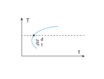
where the relative phase fraction X has been used. Note that at a fixed temperature, the equilibrium phase fraction is constant, and it can therefore be included in the rate term in Equation 3-16. The reference rate is temperature dependent (and dependent on chemical composition and grain size, in the original Kirkaldy–Venugopalan formulation). At a fixed temperature, t1 is the time to reach the destination phase fraction (or alternatively, to reach the relative phase fraction X1), see Figure 3-3. This is expressed as

Using Equation 3-16, the rate coefficient is expressed as

Note that if the retardation coefficient Cr is known, the integral can be computed a priori for a fixed X1. The rate coefficient is therefore inversely proportional to the time it takes to reach the relative phase fraction X1.

This phase transformation model was developed by Koistinen and Marburger (Ref. 2) to model the diffusionless (displacive) austenite-martensite transformation in iron-carbon alloys and carbon steels. The onset of the transformation, which only occurs on cooling, is characterized by a critical start temperature — the martensite start temperature Ms. Above this temperature, no transformation from austenite (the source phase) to martensite (the destination phase) occurs. Below Ms, the amount of formed martensite is proportional to the undercooling below Ms, given by Ms − T. On rate form, the Koistinen–Marburger equation can be written

where β is the Koistinen–Marburger coefficient. Note that the transformation of austenite into martensite only occurs below Ms and only during cooling (that is, when ). To make the onset of martensitic transformation numerically smooth, a parameter ΔMs is used. The smoothing parameter defines a smoothed Heaviside function that makes the onset of martensitic transformation gradual. The parameter should be chosen small enough that the start temperature characteristic is retained. Assuming a constant cooling rate and that the phase fraction of austenite at Ms is , the rate equation can be integrated to

This integrated form is commonly found in the literature. The rate form of Equation 3-20 is more general, and from a computational standpoint it is more suitable for implementation. The rate form is therefore used in the phase transformation interfaces.

Using this option, other types of phase transformations can be defined. A user-defined phase transformation assumes that a source phase decomposes into a destination phase according to Equation 3-1.