Optical Aberration Plot and Aberration Evaluation

The plot can be added in a whereas the node is available under . Both of these postprocessing features serve a similar purpose: to quantify the monochromatic aberrations of an imaging system and express them in terms of Zernike polynomial coefficients. In order to use the plot, the following prerequisites must be met:

•

The model component must be 3D.

•

An instance of the Geometrical Optics interface must be present and solved for.

•

The check box must be selected in the Geometrical Optics window before solving.

•

An dataset must be created. This dataset must point to a dataset. Optionally, this dataset can be automatically generated (see below). In the Settings window for the dataset, must be selected from the list. The is the location of the focus and the points from the focus toward the center of the exit pupil.

Using the hemisphere defined in the dataset, a Gaussian reference sphere is defined. The optical path difference among intersection points with this sphere is then expressed as a sum of Zernike polynomials.

Automatic Dataset Generation

Alternatively, using the plot, you can use the button in the section to automatically generate a reference hemisphere at the location of the rms focus. However, note that the defocus term Z(2,0) might be larger for the rms focus than it would for some other definitions of the image plane, such as the marginal focus.

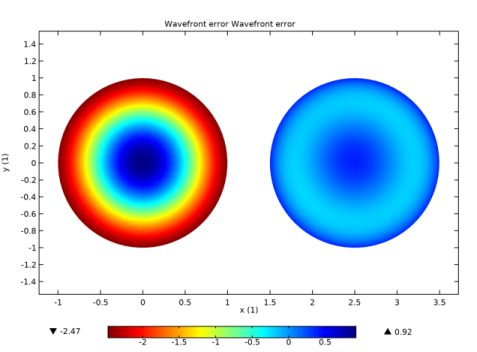
The monochromatic aberrations in a double Gauss lens system are shown in Figure 2-12. The circle on the left shows the sum of all Zernike coefficients. The circle on the right ignores the defocus term Z(2,0) and the piston term Z(0,0). Usually, lower-order Zernike terms can be reduced by correcting misalignments in the optical system or adjusting the nominal focus. Higher-order terms are consequences of the type of lens or mirror used in an optical system; for example, a single spherical lens will always demonstrate some spherical aberration, for any position of the nominal focus.

The plot always shows the optical path differences on a unit circle. The color expression is the wavefront error in microns. In the circle on the right in Figure 2-12, the largest contribution is from the spherical aberration term Z(4,0).

Figure 2-12: Monochromatic aberrations in a double Gauss lens system.


	For a list of Zernike polynomials and their derivation, see Monochromatic Aberrations and the Zernike Polynomials in Theory for the Geometrical Optics Interface.