Monochromatic Aberrations and the Zernike Polynomials
A standard way to quantify monochromatic aberrations is to express the optical path difference of all incident rays as a linear combination of Zernike polynomials. With the Ray Optics Module, the Zernike coefficients can be reported in a table using the Aberration Evaluation feature. Alternatively, a superposition of different Zernike polynomials can be shown on a unit circle using the Optical Aberration plot.
Several different standards exist for naming, normalizing, and organizing the Zernike polynomials. The approach used in this section follows the standards published by the International Organization for Standardization (ISO, Ref. 19) and the American National Standards Institute (ANSI, Ref. 20).
Each Zernike polynomial can be expressed as
where
M(mθ) is the meridional term or azimuthal term,
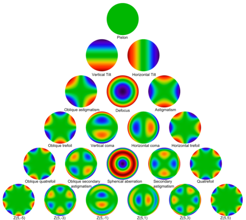
ρ is the radial parameter, given by ρ = r/a where r is the distance from the aperture center and a is the aperture radius, so that 0 ≤ ρ ≤ 1,
θ is the meridional parameter or azimuthal angle, 0 ≤ θ ≤ 2π,
the lower index n is a nonnegative integer, = 0,1,2,…, and
the upper index m is an integer, m = nn + 2, …, n − 2, n so that n − |m| is always even.
The normalization term is
where δ0,m is the Kronecker delta,
The radial term is given by the equation
where “!” denotes the factorial operator; for nonnegative integers,
The meridional term is given by the equation
The Zernike polynomials thus defined are normalized Zernike polynomials. They are orthogonal in the sense that any pair of Zernike polynomials satisfy the equation
The normalized Zernike polynomials up to fifth order, along with their common names, are given in Table 3-4.
 
Figure 3-14: Zernike polynomials on the unit circle.