2D Models

The text below is a guide to some of the common approximations made for 2D models. Remember that the modeling in 2D usually represents some 3D geometry under the assumption that nothing changes in the third dimension or that the field has a prescribed propagation component in the third dimension.

Cartesian Coordinates

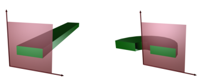
In this case a cross section is viewed in the xy-plane of the actual 3D geometry. The geometry is mathematically extended to infinity in both directions along the z-axis, assuming no variation along that axis or that the field has a prescribed wave vector component along that axis. All the total flows in and out of boundaries are per unit length along the z-axis. A simplified way of looking at this is to assume that the geometry is extruded one unit length from the cross section along the z-axis. The total flow out of each boundary is then from the face created by the extruded boundary (a boundary in 2D is a line).

There are usually two approaches that lead to a 2D cross-section view of a problem. The first approach is when it is known that there is no variation of the solution in one particular dimension.

This is shown in the model H-Bend Waveguide 2D, where the electric field only has one component in the z direction and is constant along that axis. The second approach is when there is a problem where the influence of the finite extension in the third dimension can be neglected.

Figure 2-1: The cross sections and their real geometry for Cartesian coordinates and cylindrical coordinates (axial symmetry).


	H-Bend Waveguide 2D: Application Library path RF_Module/Transmission_Lines_and_Waveguides/h_bend_waveguide_2d

Axial Symmetry (Cylindrical Coordinates)

If the 3D geometry can be constructed by revolving a cross section around an axis, and if no variations in any variable occur when going around the axis of revolution (or that the field has a prescribed wave vector component in the direction of revolution), then use an axisymmetric physics interface. The spatial coordinates are called r and z, where r is the radius. The flow at the boundaries is given per unit length along the third dimension. Because this dimension is a revolution all flows must be multiplied with αr, where α is the revolution angle (for example, 2π for a full turn).


	Conical Antenna: Application Library path RF_Module/Antennas/conical_antenna


	When using the axisymmetric versions, the horizontal axis represents the radial (r) direction and the vertical axis the z direction, and the geometry in the right half plane (that is, for positive r only) must be created.

Polarization in 2D

In addition to selecting 2D or 2D axisymmetry when you start building the model, the physics interfaces (The Electromagnetic Waves, Frequency Domain Interface or The Electromagnetic Waves, Transient Interface) in the Model Builder offers a choice in the Components settings section. The available choices are Out-of-plane vector, In-plane vector, and Three-component vector. This choice determines what polarizations can be handled. For example, as you are solving for the electric field, a 2D TM (out-of-plane H field) model requires choosing In-plane vector as then the electric field components are in the modeling plane.