PDF

Surface Cracked Cylinder
Introduction
This model reproduces a NAFEMS benchmark (Ref. 1) in which a pressurized cylinder has a horizontal semi-elliptic crack on its inner surface. The energy release rate is calculated along the crack front using the J-integral method. The stress intensity factors calculated from the J-integral are then compared to the reference data.
Model Definition
Since the model consists on a cylinder with a horizontal crack on its mid plane, only a quarter of the whole geometry is built. A tube around the elliptical crack front is built to generate a swept mesh along it. The swept mesh makes the J-integral curve along the crack front smoother.
A Symmetry condition is applied on the thickness boundaries of the cylinder. On the crack boundaries, it is overridden by a Crack feature. The crack is symmetric to define explicitly the crack front. Due to the symmetry, the stress intensity factors for modes II and III will be zero.
The pressure load can be applied with a Boundary Load feature on the inner face of the cylinder, and with the Face Load subfeature on the crack face .
The J-integral at a point of the crack front is composed of a closed contour integral and a surface integral. The closed contour integral is composed of a circular integral around the crack front and an integral on the crack face to take into account the force applied on it.
The stress intensity factor in mode I is then computed from the J-integral
where E* is the equivalent Young’s modulus. A 2D plane strain condition is assumed, so
.
Results and Discussion
Figure 1 shows the default stress plot, where a stress concentration around the crack front is visible. Figure 2 shows a closer view of this stress concentration
Figure 1: Von Mises stress in the cylinder and at the crack front.
Figure 2: Close view of the stress concentration at the crack front.
The J-integral calculated along the crack front represents the energy release rate per surface area when the crack is locally extended in the crack plane direction. The crack extension direction, the J-integral intensity and the surface contour used for integral calculation are plotted in Figure 3
Figure 3: 3D plot of J-integral: crack growth direction, intensity and contour used for the calculation.
Figure 4 plots the J-integral as function of the parametric angle along the elliptic crack. A jump in the curve at zero angle can be noticed. This glitch is often seen near free boundaries due to the singularities that contribute to the surface integral.
Figure 4: J-integral along the crack front.
From the J-integral the stress intensity factor in mode I can be calculated and compared to the benchmark in Ref. 1, see Figure 5.
Figure 5: Stress intensity factor along the crack front compared to the benchmark.
Reference
1. R. Judge and B. Mardsen, Three Dimensional Test Cases in Linear Elastic Fracture Mechanics, part 4: Surface Cracked Cylinder, NAFEMS, 1993.
Application Library path: Structural_Mechanics_Module/Fracture_Mechanics/surface_cracked_cylinder
Modeling Instructions
From the File menu, choose New.
New
In the New window, click  Model Wizard.
Model Wizard
1
In the Model Wizard window, click  3D.
2
In the Select Physics tree, select Structural Mechanics>Solid Mechanics (solid).
3
Click Add.
4
Click  Study.
5
In the Select Study tree, select General Studies>Stationary.
6
Geometry 1
1
In the Geometry toolbar, click  Insert Sequence.
2
3
In the Geometry toolbar, click  Build All.
Global Definitions
Parameters 1
1
In the Model Builder window, under Global Definitions click Parameters 1.
2
In the Settings window for Parameters, locate the Parameters section.
3
Materials
Material 1 (mat1)
1
In the Materials toolbar, click  Blank Material.
2
In the Settings window for Material, locate the Material Contents section.
3
Solid Mechanics (solid)
Symmetry 1
1
In the Model Builder window, under Component 1 (comp1) right-click Solid Mechanics (solid) and choose More Constraints>Symmetry.
2
The Symmetry condition is applied on the whole thickness of the cylinder. It will be overridden by the Crack feature on the crack surface.
Prescribed Displacement 1
1
In the Physics toolbar, click  Points and choose Prescribed Displacement.
2
3
In the Settings window for Prescribed Displacement, locate the Prescribed Displacement section.
4
Select the Prescribed in z direction check box.
Crack 1
1
In the Physics toolbar, click  Boundaries and choose Crack.
2
3
In the Settings window for Crack, locate the Crack Definition section.
4
From the Crack surface list, choose Symmetric.
5
Click to expand the Crack Front section. Click  Clear Selection.
6
J-Integral 1
In the Physics toolbar, click  Attributes and choose J-Integral.
Boundary Load 1
1
In the Physics toolbar, click  Boundaries and choose Boundary Load.
Apply pressure load on the inner face of the cylinder. The pressure on the crack will be applied under the Crack feature.
2
3
In the Settings window for Boundary Load, locate the Force section.
4
From the Load type list, choose Pressure.
5
In the p text field, type p.
Crack 1
In the Model Builder window, click Crack 1.
Face Load 1
1
In the Physics toolbar, click  Attributes and choose Face Load.
2
In the Settings window for Face Load, locate the Load section.
3
In the p text field, type p.
Mesh 1
Free Triangular 1
In the Mesh toolbar, click  Boundary and choose Free Triangular.
Size
1
In the Model Builder window, click Size.
2
In the Settings window for Size, locate the Element Size section.
3
Click the Custom button.
4
Locate the Element Size Parameters section. In the Maximum element size text field, type th/2.
5
In the Minimum element size text field, type a/200.
Free Triangular 1
1
In the Model Builder window, click Free Triangular 1.
2
Size 1
1
Right-click Free Triangular 1 and choose Size.
2
In the Settings window for Size, locate the Geometric Entity Selection section.
3
From the Geometric entity level list, choose Point.
4
5
Locate the Element Size section. Click the Custom button.
6
Locate the Element Size Parameters section. Select the Maximum element size check box.
7
8
Select the Minimum element size check box.
9
10
Select the Maximum element growth rate check box.
11
12
Click  Build Selected.
Swept 1
1
In the Mesh toolbar, click  Swept.
2
In the Settings window for Swept, locate the Domain Selection section.
3
From the Geometric entity level list, choose Domain.
4
Distribution 1
1
Right-click Swept 1 and choose Distribution.
2
In the Settings window for Distribution, locate the Distribution section.
3
From the Distribution type list, choose Predefined.
4
In the Number of elements text field, type 40.
5
In the Element ratio text field, type 6.
6
Select the Reverse direction check box.
7
Click  Build Selected.
Free Tetrahedral 1
1
In the Mesh toolbar, click  Free Tetrahedral.
2
In the Settings window for Free Tetrahedral, locate the Domain Selection section.
3
From the Geometric entity level list, choose Domain.
4
5
Click  Build Selected.
Swept 2
1
In the Mesh toolbar, click  Swept.
2
In the Settings window for Swept, locate the Domain Selection section.
3
From the Geometric entity level list, choose Domain.
4
Swept 3
In the Mesh toolbar, click  Swept.
Distribution 1
1
Right-click Swept 3 and choose Distribution.
2
In the Settings window for Distribution, locate the Distribution section.
3
From the Distribution type list, choose Predefined.
4
In the Number of elements text field, type 12.
5
In the Element ratio text field, type 4.
6
Click  Build All.
Study 1
In the Home toolbar, click  Compute.
Results
Surface 1
1
In the Model Builder window, expand the Stress (solid) node, then click Surface 1.
2
In the Settings window for Surface, locate the Expression section.
3
From the Unit list, choose MPa.
4
Click to expand the Range section. Select the Manual color range check box.
5
In the Minimum text field, type 0.
6
In the Maximum text field, type 20.
Stress (solid)
1
In the Model Builder window, click Stress (solid).
2
In the Settings window for 3D Plot Group, locate the Plot Settings section.
3
Clear the Plot dataset edges check box.
4
In the Stress (solid) toolbar, click  Plot.
The first default plot shows von Mises stress. On a closer view the maximum stress is visible along the crack front, see Figure 2.
There is also a default arrow plot that shows the crack direction and the intensity of J-integral, Figure 3. The contour used to calculate the J-integral is displayed as well.
Cracks (solid)
To plot the J-integral (Figure 4) along crack front, you may introduce the parametric angle along the ellipse.
Definitions
Variables 1
1
In the Home toolbar, click  Variables and choose Local Variables.
2
In the Settings window for Variables, locate the Geometric Entity Selection section.
3
From the Geometric entity level list, choose Domain.
4
5
Locate the Variables section. In the table, enter the following settings:
Study 1
In the Study toolbar, click  Update Solution.
Results
J-Integral 1
1
In the Model Builder window, expand the Crack 1, J-Integral (solid) node, then click J-Integral 1.
2
In the Settings window for Line Graph, locate the x-Axis Data section.
3
From the Parameter list, choose Expression.
4
In the Expression text field, type angle.
5
From the Unit list, choose °.
6
In the Crack 1, J-Integral (solid) toolbar, click  Plot.
Duplicate the last plot group to plot and compare the stress intensity factor to the reference value, Figure 5
Crack 1, KI
1
In the Model Builder window, right-click Crack 1, J-Integral (solid) and choose Duplicate.
2
In the Settings window for 1D Plot Group, type Crack 1, KI in the Label text field.
KI
1
In the Model Builder window, expand the Crack 1, KI node, then click J-Integral 1.
2
In the Settings window for Line Graph, type KI in the Label text field.
3
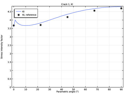
Click Replace Expression in the upper-right corner of the y-Axis Data section. From the menu, choose Component 1 (comp1)>Solid Mechanics>Cracks>solid.crack1.jint1.KI - Stress intensity factor, mode I.
4
Locate the y-Axis Data section. In the Expression text field, type solid.crack1.jint1.KI/1e6.
Crack 1, KI
1
In the Model Builder window, click Crack 1, KI.
2
In the Settings window for 1D Plot Group, locate the Plot Settings section.
3
Select the x-axis label check box.
4
Select the y-axis label check box.
5
In the associated text field, type Stress intensity factor.
6
Locate the Axis section. Select the Manual axis limits check box.
7
In the y minimum text field, type 0.
8
In the Crack 1, KI toolbar, click  Plot.
Import the stress intensity factors from benchmark to compare with the computed results.
Table 1
1
In the Results toolbar, click  Table.
2
In the Settings window for Table, locate the Data section.
3
Click Import.
4
Table Graph 1
1
Right-click Crack 1, KI and choose Table Graph.
2
In the Settings window for Table Graph, locate the Coloring and Style section.
3
From the Color list, choose From theme.
4
Find the Line style subsection. From the Line list, choose None.
5
Find the Line markers subsection. From the Marker list, choose Asterisk.
6
From the Positioning list, choose In data points.
7
In the Crack 1, KI toolbar, click  Plot.
Crack 1, KI
1
In the Model Builder window, click Crack 1, KI.
2
In the Settings window for 1D Plot Group, locate the Legend section.
3
Select the Show legends check box.
4
From the Position list, choose Upper left.
KI
1
In the Model Builder window, click KI.
2
In the Settings window for Line Graph, click to expand the Legends section.
3
Select the Show legends check box.
4
From the Legends list, choose Manual.
5
Table Graph 1
1
In the Model Builder window, click Table Graph 1.
2
In the Settings window for Table Graph, click to expand the Legends section.
3
Select the Show legends check box.
4
From the Legends list, choose Manual.
5