
|
|
|


|
1
|
|
2
|
|
3
|
Click Add.
|
|
4
|
Click
|
|
5
|
|
6
|
Click
|
|
1
|
|
2
|
|
1
|
|
2
|
|
3
|
|
4
|
|
5
|
|
6
|
|
7
|
|
1
|
|
2
|
|
3
|
|
1
|
|
2
|
|
3
|
|
1
|
In the Model Builder window, under Component 1 (comp1)>Hydrodynamic Bearing (hdb) click Hydrodynamic Journal Bearing 1.
|
|
2
|
|
3
|
|
4
|
|
5
|
|
6
|
|
7
|
|
8
|
|
9
|
Locate the Fluid Properties section. From the μ list, choose User defined. In the associated text field, type mu0.
|
|
10
|
|
1
|
|
2
|
|
3
|
|
1
|
|
3
|
|
4
|
|
1
|
|
3
|
|
4
|
|
5
|
|
1
|
|
2
|
|
3
|
|
4
|
Click
|
|
6
|
|
1
|
|
2
|
|
1
|
|
2
|
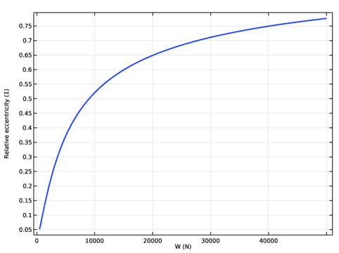
In the Settings window for Global, click Replace Expression in the upper-right corner of the y-Axis Data section. From the menu, choose Component 1 (comp1)>Hydrodynamic Bearing>Hydrodynamic Journal Bearing 1>hdb.hjb1.ec_rel - Relative eccentricity.
|
|
3
|
|
4
|
|
5
|
|
1
|
|
2
|
|
3
|
|
4
|
|
1
|
|
2
|
|
1
|
|
2
|
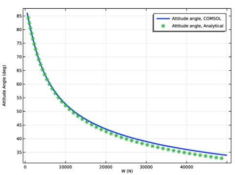
In the Settings window for Global, click Replace Expression in the upper-right corner of the y-Axis Data section. From the menu, choose Component 1 (comp1)>Hydrodynamic Bearing>Hydrodynamic Journal Bearing 1>hdb.hjb1.phia - Attitude angle - rad.
|
|
3
|
|
4
|
|
1
|
|
2
|
|
4
|
Locate the Coloring and Style section. Find the Line style subsection. From the Line list, choose None.
|
|
5
|
|
6
|
|
7
|
|
1
|
|
2
|
|
3
|
|
4
|
In the associated text field, type Attitude Angle (deg).
|
|
5
|
|
1
|
|
2
|
|
1
|
|
2
|
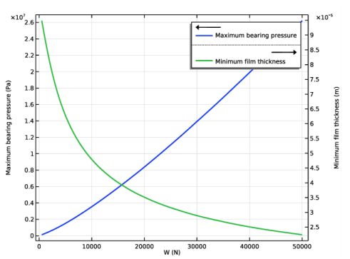
In the Settings window for Global, click Replace Expression in the upper-right corner of the y-Axis Data section. From the menu, choose Component 1 (comp1)>Hydrodynamic Bearing>Journal and bearing properties>hdb.hjb1.p_max - Maximum bearing pressure - Pa.
|
|
1
|
|
2
|
In the Settings window for Global, click Replace Expression in the upper-right corner of the y-Axis Data section. From the menu, choose Component 1 (comp1)>Hydrodynamic Bearing>Journal and bearing properties>hdb.hjb1.h_min - Minimum film thickness - m.
|
|
1
|
|
2
|
|
3
|
|
4
|
|
5
|
|
6
|
|
1
|
|
2
|
|
1
|
|
2
|
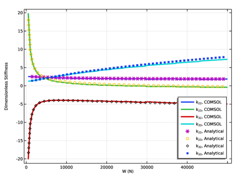
In the Settings window for Global, click Replace Expression in the upper-right corner of the y-Axis Data section. From the menu, choose Component 1 (comp1)>Hydrodynamic Bearing>Dynamic coefficients>hdb.hjb1.k22 - Bearing stiffness, local yy component - N/m.
|
|
3
|
Click Add Expression in the upper-right corner of the y-Axis Data section. From the menu, choose Component 1 (comp1)>Hydrodynamic Bearing>Dynamic coefficients>hdb.hjb1.k23 - Bearing stiffness, local yz component - N/m.
|
|
4
|
Click Add Expression in the upper-right corner of the y-Axis Data section. From the menu, choose Component 1 (comp1)>Hydrodynamic Bearing>Dynamic coefficients>hdb.hjb1.k32 - Bearing stiffness, local zy component - N/m.
|
|
5
|
Click Add Expression in the upper-right corner of the y-Axis Data section. From the menu, choose Component 1 (comp1)>Hydrodynamic Bearing>Dynamic coefficients>hdb.hjb1.k33 - Bearing stiffness, local zz component - N/m.
|
|
6
|
|
7
|
|
1
|
|
2
|
|
4
|
Locate the Coloring and Style section. Find the Line style subsection. From the Line list, choose None.
|
|
5
|
|
6
|
|
1
|
|
2
|
|
3
|
|
4
|
In the associated text field, type Dimensionless Stiffness.
|
|
5
|
|
6
|
|
1
|
|
2
|
|
1
|
|
2
|
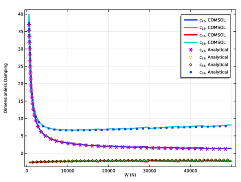
In the Settings window for Global, click Replace Expression in the upper-right corner of the y-Axis Data section. From the menu, choose Component 1 (comp1)>Hydrodynamic Bearing>Dynamic coefficients>hdb.hjb1.c22 - Bearing damping coefficient, local yy component - N·s/m.
|
|
3
|
|
4
|
|
1
|
|
2
|
|
4
|
Locate the Coloring and Style section. Find the Line style subsection. From the Line list, choose None.
|
|
5
|
|
6
|
|
7
|
|
1
|
|
2
|
|
3
|
|
4
|
|
5
|
In the associated text field, type Dimensionless Damping.
|