|
|
|
|
Nominal x field angle
|
||
|
Nominal y field angle
|
||
|
|
||
|
Number of x fields
|
||
|
Number of y fields
|
||
|
x field step
|
||
|
y field step
|
||
|
Minimum x field
|
||
|
|
Maximum x field
|
|
|
Minimum y field
|
||
|
|
Maximum y field
|
|
Ray direction vector, x-component
|
||
|
Ray direction vector, y-component
|
||
|
Ray direction vector, z-component
|
||
 |
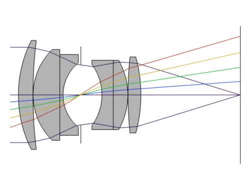
Stop z-coordinate, where Tc,n is the central thickness of element n and Tn is the separation between elements n and n+1. Note that the stop is the 4th element in the Double Gauss lens
|
|
 |
Image plane z-coordinate, where Tc,n is the central thickness of element n and Tn is the separation between elements n and n+1. Including the stop, the Double Gauss lens has 7 elements.
|
|
|
Pupil shift, x-coordinate
|
||
|
Pupil shift, y-coordinate
|
|
1
|
|
2
|
|
3
|
Click Add.
|
|
4
|
Click
|
|
5
|
|
6
|
Click
|
|
1
|
|
2
|
In the Settings window for Parameters, type Parameters 1: Lens Prescription in the Label text field.
|
|
1
|
|
2
|
|
3
|
|
4
|
Browse to the model’s Application Libraries folder and double-click the file double_gauss_lens_parametric_parameters.txt.
|
|
1
|
|
2
|
|
3
|
Find the Mesh frame coordinates subsection. From the Geometry shape function list, choose Cubic Lagrange. The ray tracing algorithm used by the Geometrical Optics interface computes the refracted ray direction based on a discretized geometry via the underlying finite element mesh. A cubic geometry shape order usually introduces less discretization error compared to the default, which uses linear and quadratic polynomials.
|
|
1
|
|
2
|
|
3
|
|
4
|
|
5
|
Browse to the model’s Application Libraries folder and double-click the file double_gauss_lens_parametric_variables.txt.
|
|
1
|
|
2
|
|
3
|
|
4
|
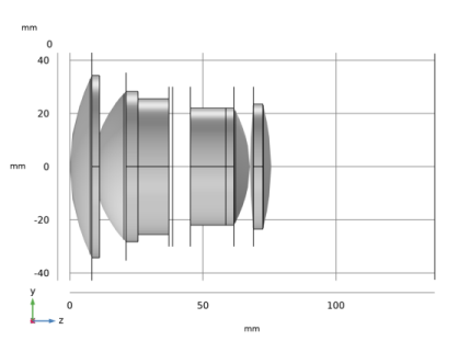
Browse to the model’s Application Libraries folder and double-click the file double_gauss_lens_geom_sequence.mph.
|
|
5
|
|
6
|
Click the
|
|
7
|
|
1
|
|
2
|
|
3
|
|
4
|
|
5
|
|
6
|
|
7
|
|
8
|
|
9
|
|
1
|
|
2
|
|
3
|
From the Selection list, choose Lens Material 1. Each of the 6 lenses has been assigned to one of three lens material selections.
|
|
1
|
|
2
|
|
3
|
|
1
|
|
2
|
|
3
|
|
1
|
|
2
|
|
3
|
In the Maximum number of secondary rays text field, type 0. In this simulation stray light is not being traced, so reflected rays will not be produced at the lens surfaces.
|
|
4
|
Select the Use geometry normals for ray-boundary interactions check box. In this simulation, the geometry normals are used to apply the boundary conditions on all refracting surfaces. This is appropriate for the highest accuracy ray traces in single-physics simulations, where the geometry is not deformed.
|
|
5
|
|
6
|
|
7
|
|
1
|
In the Model Builder window, under Component 1 (comp1)>Geometrical Optics (gop) click Medium Properties 1.
|
|
2
|
|
3
|
From the Optical dispersion model list, choose Get dispersion model from material. Each of the materials added above contain the optical dispersion coefficients which can be used to compute the refractive index as a function of wavelength.
|
|
1
|
|
2
|
|
3
|
|
1
|
|
2
|
|
3
|
In the λ0 text field, type lam_vac. This wavelength was defined in the Parameters node. It will be updated during the Parameteric Sweep.
|
|
1
|
|
2
|
|
3
|
|
4
|
|
5
|
|
6
|
|
7
|
|
8
|
|
1
|
|
2
|
|
3
|
|
4
|
|
1
|
|
2
|
|
3
|
|
4
|
|
1
|
|
2
|
|
3
|
Locate the Boundary Selection section. From the Selection list, choose Image Plane. The default Wall condition (Freeze) will be used.
|
|
1
|
|
2
|
|
3
|
|
4
|
|
1
|
|
2
|
|
3
|
|
4
|
Click
|
|
5
|
Click
|
|
1
|
|
2
|
|
3
|
|
4
|
|
5
|
In the Lengths text field, type 0 200. The maximum optical path length is sufficient for rays released at large field angles to reach the image plane.
|
|
6
|
|
1
|
|
2
|
|
3
|
|
4
|
|
1
|
|
2
|
|
3
|
|
4
|
|
5
|
|
1
|
|
2
|
|
3
|
|
4
|
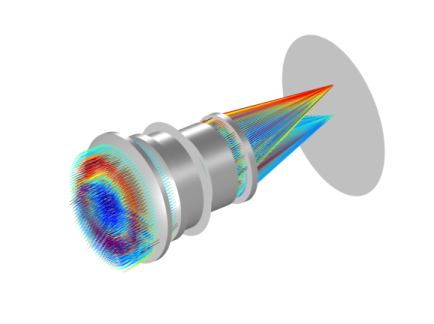
Locate the Plot Settings section. Clear the Plot dataset edges check box. The lenses will be rendered using a Mesh plot.
|
|
1
|
|
2
|
|
3
|
|
4
|
|
5
|
|
1
|
|
2
|
|
3
|
|
4
|
|
5
|
|
1
|
|
2
|
|
3
|
|
1
|
|
2
|
|
3
|
|
1
|
|
2
|
|
3
|
|
4
|
|
5
|
|
6
|
|
1
|
|
2
|
|
3
|
|
1
|
|
2
|
|
3
|
|
4
|
|
1
|
|
2
|
|
3
|
|
4
|
Click to expand the Inherit Style section. From the Plot list, choose Ray Trajectories 1. This step only needs to be taken on the first duplication.
|
|
1
|
|
2
|
|
3
|
|
1
|
|
2
|
|
3
|
|
4
|
|
1
|
|
2
|
|
3
|
|
1
|
|
2
|
|
3
|
|
1
|
|
2
|
|
3
|
|
4
|
|
5
|
|
6
|
|
7
|
|
8
|
|
1
|
|
2
|
|
3
|
|
4
|
|
5
|
|
1
|
|
2
|
|
3
|
|
4
|
|
5
|
|
6
|
|
7
|
|
8
|
|
1
|
In the Model Builder window, under Results>Spot Diagram 1 right-click Poincaré Map 1 and choose Duplicate.
|
|
2
|
|
3
|
|
4
|
|
1
|
|
2
|
|
3
|
|
1
|
|
2
|
|
3
|
|
4
|
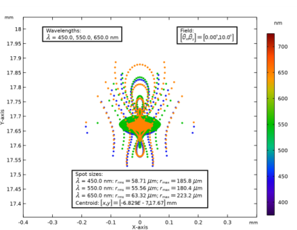
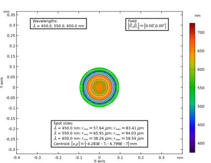
Locate the Annotation section. In the Text text field, type Wavelengths: \\ $\lambda$ = eval(lam1/1[nm]), eval(lam2/1[nm]), eval(lam3/1[nm]) nm.
|
|
5
|
|
6
|
|
7
|
|
8
|
|
9
|
|
10
|
|
11
|
|
12
|
|
1
|
|
2
|
|
3
|
In the Text text field, type Field: \\ $\left[\theta_\textrm{x},\theta_\textrm{y}\right] = \left[eval(theta_x0/1[deg])^\circ,eval(theta_y0/1[deg])^\circ\right]$.
|
|
4
|
|
5
|
|
6
|
|
1
|
|
2
|
|
3
|
In the Text text field, type Spot sizes: \\ $\lambda$ = eval(lam1/1[nm]) nm: $r_\textrm{rms} = eval(1e3*r_rms0_1)~\mu$m; $r_\textrm{max} = eval(r_max0_1/1[um])~\mu$m \\ $\lambda$ = eval(lam2/1[nm]) nm: $r_\textrm{rms} = eval(1e3*r_rms0_2)~\mu$m; $r_\textrm{max} = eval(r_max0_2/1[um])~\mu$m \\ $\lambda$ = eval(lam3/1[nm]) nm: $r_\textrm{rms} = eval(1e3*r_rms0_3)~\mu$m; $r_\textrm{max} = eval(r_max0_3/1[um])~\mu$m \\ Centroid: $[x,y] = [eval(qx_ave0),eval(qy_ave0)]$ mm.
|
|
4
|
|
5
|
|
6
|
|
7
|
|
8
|
|
1
|
|
2
|
|
1
|
|
2
|
|
3
|
|
1
|
|
2
|
|
3
|
|
1
|
|
2
|
|
3
|
|
1
|
|
2
|
|
3
|
|
4
|
|
1
|
|
2
|
|
3
|
In the Text text field, type Field: \\ $\left[\theta_\textrm{x},\theta_\textrm{y}\right] = \left[eval(theta_x1/1[deg])^\circ,eval(theta_y1/1[deg])^\circ\right]$.
|
|
4
|
|
5
|
|
1
|
|
2
|
|
3
|
In the Text text field, type Spot sizes: \\ $\lambda$ = eval(lam1/1[nm]) nm: $r_\textrm{rms} = eval(1e3*r_rms1_1)~\mu$m; $r_\textrm{max} = eval(r_max1_1/1[um])~\mu$m \\ $\lambda$ = eval(lam2/1[nm]) nm: $r_\textrm{rms} = eval(1e3*r_rms1_2)~\mu$m; $r_\textrm{max} = eval(r_max1_2/1[um])~\mu$m \\ $\lambda$ = eval(lam3/1[nm]) nm: $r_\textrm{rms} = eval(1e3*r_rms1_3)~\mu$m; $r_\textrm{max} = eval(r_max1_3/1[um])~\mu$m \\ Centroid: $[x,y] = [eval(qx_ave1),eval(qy_ave1)]$ mm.
|
|
4
|
|
5
|
|
6
|