Double Gauss Lens

A double Gauss lens is a multiple element objective lens commonly used in imaging systems. It is capable of high quality imagery over moderately large field angles, at modest to high speed. In this tutorial, a double Gauss lens model (Figure 1) is constructed using multiple instances of standard parts from the built-in Part Library for the Ray Optics Module. The results of a ray trace will be presented together with a spot diagram and a wavefront aberration diagram.

Figure 1: Overview of the double Gauss lens used in this tutorial. In this view the marginal rays of an on-axis trace are shown, together with the chief ray of 4 additional fields.

Model Definition

The double Gauss lens simulated in this tutorial is an f/1.7, 100.2 mm focal length, 19° field of view lens by Lautebacher & Brendel (Agfa Camera Werk Ag, U.S. Patent 2784643), from Ref. 1, p. 323. The prescription of this lens is given in Table 1 and the instructions for creating the lens can be found in the Appendix — Geometry Instructions.

The lens geometry is created by inserting each lens element (including the stop) sequentially, such that each subsequent lens is placed relative to the prior one. This process is simplified by making use of the predefined work planes within the part instances. It is important to appreciate that the ray tracing method used by the Geometrical Optics interface is inherently nonsequential, so the same result could be obtained by placing part instances within the geometry in any order. The double Gauss lens geometry sequence is shown in Figure 2 and the default, Physics-controlled mesh, is seen in Figure 3.

In addition to the lens parameters used to define the lens geometry, a set of parameters are required to define the ray trace. These are detailed in Table 2.

Table 1: DouBLE Gauss lens parameters.
Index	Name	Radius (mm)	Thickness (mm)	Material	Clear radius (mm)
—	Object	∞	∞	—	—
1	Lens 1	75.050	9.000	LaF3	33.0
—	—	270.700	0.100	—	33.0
2	Lens 2	39.270	16.510	BaF11	27.5
3	Lens 3	∞	2.000	N-SF5	24.5
—	—	25.650	10.990	—	19.5
4	Stop	∞	13.000	—	18.6
5	Lens 4	−31.870	7.030	N-SF5	18.5
6	Lens 5	∞	8.980	LaF3	21.0
—	—	−43.510	0.100	—	21.0
7	Lens 6	221.140	7.980	BaF11	23.0
—	—	−88.790	61.418	—	23.0
—	Image	∞	—	—	42.5

Table 2: Global parameter definitions.
Parameter	Value	Description
λvac	550 nm	Nominal (vacuum) wavelength
θx	0°	Nominal x field angle
θy	0°	Nominal y field angle
Nring	18	Number of hexapolar rings. (Nring = 18 will give a total of 1027 rays.)
Pnom	58.941 mm	Nominal entrance pupil diameter
Pfac1	−1.15	Pupil shift factor 1
Pfac2	−0.60	Pupil shift factor 2

Figure 2: The double Gauss lens geometry sequence.

Figure 3: The default Physics-controlled mesh for the double Gauss lens.

Several of the parameters defined in Table 2 are used to derive additional parameters such as the ray direction vector components, the stop and image plane z-coordinates, as well as the entrance pupil location. Table 3 gives the expressions used to derived these parameters. Note that the pupil shift factor is used in a empirical approximation to ensure that the chief ray passes through the center of the stop at all field angles.

Table 3: Global parameter definitions (Derived).
Parameter	Value	Description
vx	tan θx	Ray direction vector, x-component
vy	tan θy	Ray direction vector, y-component
vz	1	Ray direction vector, z-component
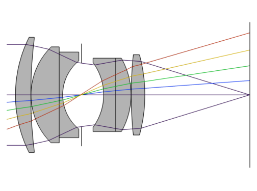
zstop		Stop z-coordinate, where Tc,n is the central thickness of element n and Tn is the separation between elements n and n+1. Note that the stop is the 4th element in the double Gauss lens.
zimage		Image plane z-coordinate, where Tc,n is the central thickness of element n and Tn is the separation between elements n and n+1. Including the stop, the double Gauss lens has 7 elements.
Pfac	Pfac1 + Pfac2 sinθ	Pupil shift factor, where
Δxpupil	(Δzpupil + Pfac zstop)tan θx	Pupil shift, x-coordinate
Δypupil	(Δzpupil + Pfac zstop)tan θy	Pupil shift, y-coordinate

Results and Discussion

A ray trace has been made at a single wavelength (550 nm) and field angle (on-axis). In Figure 4 the ray trajectories can be seen colored by optical path length and in Figure 5, a color expression based on the location of the rays at the image plane is used.

Spot diagrams at both the nominal and refocused image plane are shown in Figure 6. The refocused spot diagram in Figure 6 uses an dataset which has been automatically positioned on the plane which minimizes the RMS spot size. At this wavelength and field angle, this plane is located 187 μm ahead of the nominal image surface.

Figure 7 shows the wavefront error. After removing piston and defocus, it is possible to see that spherical aberration dominates the remaining terms.

Figure 4: Ray diagram of the double Gauss lens colored by optical path length.

Figure 5: Ray diagram of the double Gauss lens where the rays are colored by their radial distance from the centroid on the image plane.

Figure 6: Spot diagram for the double Gauss lens. The spot on the nominal image plane is on the left, and the spot on the “best focus” plane is seen on the right.

Figure 7: The double Gauss lens optical aberration diagram. The plot on the left uses all Zernike terms. On the right, piston and defocus are removed.

Reference

1. W.J. Smith, Modern lens design, vol. 2. New York, NY, USA: McGraw-Hill, 2005.

Ray_Optics_Module/Lenses_Cameras_and_Telescopes/double_gauss_lens

Modeling Instructions

From the menu, choose .

New

In the window, click

Model Wizard

In the window, click

In the tree, select .

Click .

Click

In the tree, select .

Click

Global Definitions

Parameters 1: Lens Prescription

In the window, under click .

In the window for , type Parameters 1: Lens Prescription in the text field.

. The lens prescription will be added when the geometry sequence is inserted in the following section.

Parameters 2: General

The double Gauss lens simulation parameters can be loaded from a text file.

In the toolbar, click

and choose .

In the window for , type Parameters 2: General in the text field.

Locate the section. Click

Browse to the model’s Application Libraries folder and double-click the file double_gauss_lens_parameters.txt.

Component 1 (comp1)

In the window, click .

In the window for , locate the section.

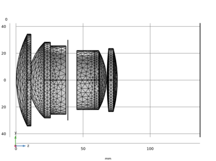
Find the subsection. From the list, choose . The ray tracing algorithm used by the Geometrical Optics interface computes the refracted ray direction based on a discretized geometry via the underlying finite element mesh. A cubic geometry shape order usually introduces less discretization error compared to the default, which uses linear and quadratic polynomials.

Double Gauss Lens

Insert the prepared geometry sequence from file. You can read the instructions for creating the geometry in the appendix. Following insertion, the lens definitions will be available in the node.

In the window, under click .

In the window for , type Double Gauss Lens in the text field.

In the toolbar, click

Browse to the model’s Application Libraries folder and double-click the file double_gauss_lens_geom_sequence.mph.

In the toolbar, click

Click the

button in the toolbar.

Click the

button in the toolbar. Orient the view to place the z-axis (optical axis) horizontal and the y-axis vertical. Compare the resulting geometry to Figure 2.

Materials

Load the materials used by each of the lenses.

Add Material

In the toolbar, click

to open the window. Each of the 6 lenses has been assigned to one of three lens material selections.

Go to the window.

In the tree, select .

Click in the window toolbar.

In the tree, select .

Click in the window toolbar.

In the tree, select .

Click in the window toolbar.

In the toolbar, click

to close the window.

Materials

Hoya LAF3 (mat1)

In the window, under click .

In the window for , locate the section.

From the list, choose .

Hoya BAF11 (mat2)

In the window, click .

In the window for , locate the section.

From the list, choose .

Schott N-SF5 (mat3)

In the window, click .

In the window for , locate the section.

From the list, choose .

Geometrical Optics (gop)

In the window, under click .

In the window for , locate the section.

In the text field, type 0. In this simulation stray light is not being traced, so reflected rays will not be produced at the lens surfaces.

Select the check box. This ensures that geometry normals are used to apply the boundary conditions on all refracting surfaces. This is appropriate for the highest accuracy ray traces in single-physics simulations, where the geometry is not deformed.

Locate the section. From the list, choose . It is assumed that the double Gauss lens is surrounded by air at room temperature.

Locate the section. Select the check box. The optical path length will be used to create an plot.

Medium Properties 1

In the window, under click .

In the window for , locate the section.

From the list, choose . Each of the materials added above contain the optical dispersion coefficients which can be used to compute the refractive index as a function of wavelength.

Material Discontinuity 1

In the window, click .

In the window for , locate the section.

From the list, choose .

Ray Properties 1

In the window, click .

In the window for , locate the section.

In the λ0 text field, type lambda. This wavelength is defined in the node.

Release from Grid 1

Release the rays from a hexapolar grid, using the quantities defined in the node.

In the toolbar, click

and choose .

In the window for , locate the section.

From the list, choose .

Specify the qc vector as


dx	x
dy	y
dz	z

The of the hexapolar grid will change according to the field angle.

Specify the rc vector as


nix	x
niy	y
niz	z

The is the same as the global optical axis.

In the Rc text field, type P_nom/2.

In the Nc text field, type N_ring.

Locate the section. Specify the L0 vector as


vx	x
vy	y
vz	z

The is calculated using the field angles defined in the node.

Obstructions

In the toolbar, click

and choose .

In the window for , type Obstructions in the text field.

Locate the section. From the list, choose .

Stop

In the toolbar, click

and choose .

In the window for , type Stop in the text field.

Locate the section. From the list, choose .

Image

In the toolbar, click

and choose .

In the window for , type Image in the text field.

Locate the section. From the list, choose . The default () will be used.

Mesh 1

In the window, under right-click and choose . The default physics-controlled mesh settings can be used in this simulation. The mesh should look like Figure 3.

Study 1

Step 1: Ray Tracing

In the window, under click .

In the window for , locate the section.

From the list, choose .

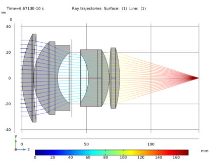
In the text field, type 0 200. The maximum optical path length is sufficient for rays released at large field angles to reach the image plane.

In the toolbar, click

Results

In the following steps, two different ray diagrams are created, one of which uses a custom color expression. Begin by making some modifications to the default ray trajectory plot. First, define a cut plane which can be used to render the double Gauss lens cross-section.

Cut Plane 1

In the toolbar, click

Ray Diagram 1

In the window, under click .

In the window for , type Ray Diagram 1 in the text field.

Locate the section. Select the check box.

From the list, choose .

In the window, expand the node.

Filter 1

In the window, expand the node, then click .

In the window for , locate the section.

From the list, choose .

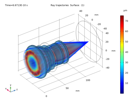
In the text field, type at(0,abs(gop.deltaqx) < 0.1[mm]). Only the sagittal rays are shown in this view.

In the following steps, the cross-section of the lens is rendered.

Surface 1

In the window, right-click and choose .

In the window for , locate the section.

From the list, choose .

Locate the section. From the list, choose .

From the list, choose .

Line 1

Right-click and choose .

In the window for , locate the section.

From the list, choose .

Locate the section. From the list, choose .

From the list, choose .

In the toolbar, click

. Compare the resulting image to Figure 4.

Ray Diagram 2

For the second ray diagram the rays will be colored according to the radial distance from the ray’s location in the image plane to the centroid. This makes it possible to visualize which rays are contributing to the image plane spot aberrations.

In the toolbar, click

and choose .

In the window for , type Ray Diagram 2 in the text field.

Locate the section. From the list, choose .

Locate the section. Select the check box.

Ray Trajectories 1

In the toolbar, click

and choose .

Color Expression 1

Right-click and choose .

In the window for , locate the section.

In the text field, type at('last',gop.rrel). This is the radial coordinate relative to the centroid of each release feature at the image plane.

From the list, choose .

Surface 1

In the window, right-click and choose .

In the window for , locate the section.

From the list, choose .

On Windows, click the colored bar underneath, or — if you are running the cross-platform desktop — the button.

Click .

Set the RGB values to 54, 140, and 203, respectively.

Click .

Click or on the cross-platform desktop.

Selection 1

Right-click and choose .

In the window for , locate the section.

From the list, choose .

Transparency 1

In the window, right-click and choose .

In the toolbar, click

Click the

button in the toolbar.

Click the

button in the toolbar. Orient the view to match Figure 5 so that the color expression in the object plane can be clearly seen.

Spot Diagram

In the following steps, a spot diagram is created.

Spot Diagram

In the toolbar, click

and choose .

In the window for , type Spot Diagram in the text field.

Locate the section. Select the check box.

From the list, choose .

Spot Diagram 1

In the toolbar, click

and choose .

In the window for , click to expand the section.

Select the check box.

From the list, choose . Using the coordinate system allows the z coordinate to be displayed.

In the text field, type 6.

Color Expression 1

Right-click and choose .

In the window for , locate the section.

In the text field, type at(0,gop.rrel). This is the radial coordinate relative to the center at the location of the ray release.

The first spot diagram shows the intersection of the rays with the nominal image plane. This surface has been positioned so as to give the best image quality over a large range of field angles when using polychromatic light. A second spot diagram can be generated automatically on the plane which minimizes the RMS spot size for a selected field angle and wavelength.

Spot Diagram 2

In the window, under right-click and choose .

In the window for , click to expand the section.

From the list, choose . In this model, the image plane is assumed to be tangential to the optical axis which is also the z-axis.

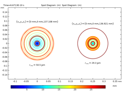
Click . This creates an dataset on a Plane. In this model, which has a single on-axis field and monochromatic light, the location of the best focus plane happens to be in front of the nominal image surface. If the best focus plane lies behind the image plane, then the condition on the defining the Image surface should be disabled. Note that the focal plane is located 187 microns in front of the nominal image surface.

Click to expand the section. In the text field, type 0.25.

Click to expand the section. From the list, choose .

In the toolbar, click

Click the

button in the toolbar. Compare the resulting image to Figure 6.

Optical Aberration Diagram

In the following steps, an optical aberration diagram is created.

Optical Aberration Diagram

In the toolbar, click

and choose .

In the window for , type Optical Aberration Diagram in the text field.

Locate the section. Select the check box.

From the list, choose .

Optical Aberration 1

In the toolbar, click

and choose .

In the window for , locate the section.

From the list, choose . As with the Spot Diagram, the image plane is assumed to be tangential to the optical axis which is also the z-axis.

Click . This creates an dataset on a reference hemisphere.

Locate the section. Select the check box.

Optical Aberration 2

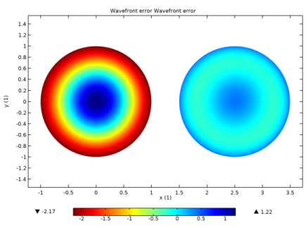
Right-click and choose . Duplicate this Aberration plot so that some Zernike terms can be removed.

In the window for , locate the section.

From the list, choose .

Click .

Clear the check box.

Clear the check box. The piston and defocus terms are removed.

Locate the section. In the text field, type 2.5.

Click to expand the section. From the list, choose .

In the toolbar, click

Click the

button in the toolbar. Compare the resulting image to Figure 7. The remaining wavefront error (about 0.6 waves) is dominated by spherical aberration.

Appendix — Geometry Instructions

From the menu, choose .

In the window, click

In the window, click

The detailed parameters of the lens can be imported from a text file. This lens is from Ref. 1, pg 323.

Parameters 1

In the window, under click .

In the window for , locate the section.

Click

Browse to the model’s Application Libraries folder and double-click the file double_gauss_lens_geom_sequence_parameters.txt.

Double Gauss Lens Parameters

The parameters that define the Double Gauss Lens geometry sequence are found in double_gauss_lens_geom_sequence_parameters.txt. These will be described in the tables below.

First, define the global optical axis. This is used to orient the first lens only. The orientation of each subsequent lens will be relative to the preceding one.


Parameter	Description
nix	Global optical axis, x-component
niy	Global optical axis, y-component
niz	Global optical axis, z-component

Next, define the parameters for each of the lens elements. Each lens requires 8 parameters in addition to the local optical axis definition (which, by convention, is coincident with the local z-axis).


Parameter	Description
R1_[n]	Radius of curvature, surface 1, lens [n]
R2_[n]	Radius of curvature, surface 2, lens [n]
Tc_[n]	Center thickness, lens [n]
d0_[n]	Outer diameter, lens [n]
d1_[n]	Diameter, surface 1, lens [n]
d2_[n]	Diameter, surface 2, lens [n]
d1_clear_[n]	Clear aperture diameter, surface 1, lens [n]
d2_clear_[n]	Clear aperture diameter, surface 2, lens [n]

Finally, define the remaining lens parameters.


Parameter	Description
T_[n]	Distance between lens elements [n] and [n+1].
d0_S	Stop maximum (outer) diameter
d1_S	Stop minimum (clear) diameter
d0_D	Diameter of image plane

Double Gauss Lens Geometry Sequence

Start constructing the lens geometry.

In the window, under click .

In the window for , type Double Gauss Lens Geometry Sequence in the text field.

Locate the section. From the list, choose .

Insert the first of the Double Gauss Lens elements.

Part Libraries

In the toolbar, click

and choose .

In the window, select in the tree.

Click

In the dialog box, select in the list.

Click . This part is used for each of the 6 Double Gauss Lens elements.

Double Gauss Lens Geometry Sequence

Lens 1

In the window, under click .

In the window for , type Lens 1 in the text field.

Locate the section. Click

Browse to the model’s Application Libraries folder and double-click the file double_gauss_lens_geom_sequence_lens1.txt. The files double_gauss_lens_geom_sequence_lens[m,m=1..6].txt contains references to each of the individual lens parameters. This avoids having to enter the values manually.

Click

Click the

button in the toolbar.

Click the

button in the toolbar. Switch the view to orthographic, and orientate the view to place the optical axis (z-axis) horizontal and the y-axis vertical.

Create cumulative selections defining the materials, clear apertures, obstructions and image plane that can be used within the final ray trace.

Cumulative Selections

In the toolbar, click

and choose .

Lens Material 1

Right-click and choose .

In the window for , type Lens Material 1 in the text field.

Lens Material 2

In the window, right-click and choose .

In the window for , type Lens Material 2 in the text field.

. In the same manner, add selections for Lens Material 3, Clear Apertures, Obstructions, Aperture Stop, and Image Plane.

Lens 1 (pi1)

Now, apply these selections.

In the window, click .

In the window for , click to expand the section.

In the table, enter the following settings:


Name	Keep	Physics	Contribute to
All		√	Lens Material 1

Click to expand the section. In the table, enter the following settings:


Name	Keep	Physics	Contribute to
Exterior		√	Lens Exteriors
Surface 1		√	Clear Apertures
Surface 2		√	Clear Apertures
Surface 1 obstruction		√	Obstructions
Surface 2 obstruction		√	Obstructions
Edges		√	Obstructions

Lens 2

Continue constructing the lens. Add the second lens element.

In the toolbar, click

and choose .

In the window for , type Lens 2 in the text field.

Locate the section. Click

Browse to the model’s Application Libraries folder and double-click the file double_gauss_lens_geom_sequence_lens2.txt.

Each lens element can be positioned in the geometry by referencing it to an existing work plane. For this example, use a work plane that is defined by the intersection of a plane tangential to the optical axis with the vertex on the exit surface of the preceding lens element.

Locate the section. Find the subsection. From the list, choose .

From the list, choose .

Find the subsection. In the text field, type T_1. This is the distance along the optical axis between the vertex on the exit surface of lens 1 and the vertex on the entrance surface of lens 2.

Locate the section. In the table, enter the following settings:


Name	Keep	Physics	Contribute to
All		√	Lens Material 2

Locate the section. In the table, enter the following settings:


Name	Keep	Physics	Contribute to
Exterior		√	Lens Exteriors
Surface 1		√	Clear Apertures
Surface 2		√	Clear Apertures
Surface 1 obstruction		√	Obstructions
Surface 2 obstruction		√	Obstructions
Edges		√	Obstructions

Lens 3

The remaining lenses are similarily defined. Next, add the third lens element.

In the toolbar, click

and choose .

In the window for , type Lens 3 in the text field.

Locate the section. Click

Browse to the model’s Application Libraries folder and double-click the file double_gauss_lens_geom_sequence_lens3.txt.

Locate the section. Find the subsection. From the list, choose .

From the list, choose .

Find the subsection. In the text field, type T_2.

Locate the section. In the table, enter the following settings:


Name	Keep	Physics	Contribute to
All		√	Lens Material 3

Locate the section. In the table, enter the following settings:


Name	Keep	Physics	Contribute to
Exterior		√	Lens Exteriors
Surface 1		√	Clear Apertures
Surface 2		√	Clear Apertures
Surface 1 obstruction		√	Obstructions
Surface 2 obstruction		√	Obstructions
Edges		√	Obstructions

Part Libraries

Next, insert the aperture stop.

In the toolbar, click

and choose .

In the window, select in the tree.

Click

. This part is also used to define the image plane and additional obstructions.

Double Gauss Lens Geometry Sequence

Stop

In the window, under click .

In the window for , type Stop in the text field.

Locate the section. In the table, enter the following settings:


Name	Expression	Value	Description
d0	d0_S	60 mm	Diameter, outer
d1	d1_S	37.2 mm	Diameter, inner
nix	0	0	Local optical axis, x-component
niy	0	0	Local optical axis, y-component
niz	1	1	Local optical axis, z-component

Locate the section. Find the subsection. From the list, choose .

From the list, choose .

Find the subsection. In the text field, type T_3+Tc_4.

Locate the section. In the table, enter the following settings:


Name	Keep	Physics	Contribute to
All		√	Aperture Stop

Lens 4

Next, add the fourth lens element.

In the toolbar, click

and choose .

In the window for , type Lens 4 in the text field.

Locate the section. Click

Browse to the model’s Application Libraries folder and double-click the file double_gauss_lens_geom_sequence_lens4.txt.

Locate the section. Find the subsection. From the list, choose .

From the list, choose .

Find the subsection. In the text field, type T_4.

Locate the section. In the table, enter the following settings:


Name	Keep	Physics	Contribute to
All		√	Lens Material 3

Locate the section. In the table, enter the following settings:


Name	Keep	Physics	Contribute to
Exterior		√	Lens Exteriors
Surface 1		√	Clear Apertures
Surface 2		√	Clear Apertures
Surface 1 obstruction		√	Obstructions
Surface 2 obstruction		√	Obstructions
Edges		√	Obstructions

Lens 5

Next, add the fifth lens element.

In the toolbar, click

and choose .

In the window for , type Lens 5 in the text field.

Locate the section. Click

Browse to the model’s Application Libraries folder and double-click the file double_gauss_lens_geom_sequence_lens5.txt.

Locate the section. Find the subsection. From the list, choose .

From the list, choose .

Find the subsection. In the text field, type T_5.

Locate the section. In the table, enter the following settings:


Name	Keep	Physics	Contribute to
All		√	Lens Material 1

Locate the section. In the table, enter the following settings:


Name	Keep	Physics	Contribute to
Exterior		√	Lens Exteriors
Surface 1		√	Clear Apertures
Surface 2		√	Clear Apertures
Surface 1 obstruction		√	Obstructions
Surface 2 obstruction		√	Obstructions
Edges		√	Obstructions

Lens 6

Add the final (sixth) lens element.

In the toolbar, click

and choose .

In the window for , type Lens 6 in the text field.

Locate the section. Click

Browse to the model’s Application Libraries folder and double-click the file double_gauss_lens_geom_sequence_lens6.txt.

Locate the section. Find the subsection. From the list, choose .

From the list, choose .

Find the subsection. In the text field, type T_6.

Locate the section. In the table, enter the following settings:


Name	Keep	Physics	Contribute to
All		√	Lens Material 2

Locate the section. In the table, enter the following settings:


Name	Keep	Physics	Contribute to
Exterior		√	Lens Exteriors
Surface 1		√	Clear Apertures
Surface 2		√	Clear Apertures
Surface 1 obstruction		√	Obstructions
Surface 2 obstruction		√	Obstructions
Edges		√	Obstructions

Image

Now, add a surface to define the image plane.

In the toolbar, click

and choose .

In the window for , type Image in the text field.

Locate the section. In the table, enter the following settings:


Name	Expression	Value	Description
d0	d0_D	85 mm	Diameter, outer
d1	0	0 m	Diameter, inner
nix	0	0	Local optical axis, x-component
niy	0	0	Local optical axis, y-component
niz	1	1	Local optical axis, z-component

Locate the section. Find the subsection. From the list, choose .

From the list, choose .

Find the subsection. In the text field, type T_7.

Locate the section. In the table, enter the following settings:


Name	Keep	Physics	Contribute to
All		√	Image Plane

Click

Click the

button in the toolbar. Compare the resulting image to Figure 2.