PDF

Specific Absorption Rate (SAR) in the Human Brain
Introduction
Scientists use the SAR (specific absorption rate) to determine the amount of radiation that human tissue absorbs. This measurement is especially important for mobile telephones, which radiate close to the brain. The model studies how a human head absorbs a radiated wave from an antenna and the temperature increase that the absorbed radiation causes.
Note: This example requires the RF Module and the Heat Transfer Module.
The increasing use of wireless equipment has also increased the amount of radiation energy to which human bodies are exposed, and it is particularly important to avoid radiation into the brain. Experts continue to debate how dangerous this radiation might be. Almost everyone agrees, however, that it is important to minimize exposure to radiation. A common property that measures absorbed energy is the SAR value, calculated as
where σ is the conductivity of human brain tissue, ρ is the density, and |E| is the norm of the electric field (RMS). The SAR value is an average over a region of either 10 g or 1 g of brain tissue, depending on national rules. This example does not calculate the average value and so it refers to the local SAR value. The maximum local SAR value is always higher than the maximum SAR value.
Model Definition
The human head geometry is the same geometry (SAM Phantom) provided by IEEE, IEC, and CENELEC from their standard specification of SAR value measurements. The original geometry was imported into COMSOL Multiphysics after minor adjustments of the original geometry.
In addition, the model samples some material parameters with a volumetric interpolation function that estimates the variation of tissue type inside the head. The source data for this function comes directly from a file named sar_in_human_head_interp.txt. That data file was created from a magnetic-resonance image (MRI) of a human head; these images contain 109 slices, each with 256-by-256 voxels (Ref. 2). The use of the variation of the data in this file on the tissue material parameters has no scientific background, and this example simply implements it to illustrate a variation in conductivity, permittivity (Figure 1), and perfusion rate as a function of the position inside the head. The model reduces the resolution of the volumetric data to 55-by-50-by-50 interpolation points, which matches the mesh-element density inside the head. Prior to generating the data file, the modeler in this case scaled, translated, and rotated the 3D MRI data to match the form of the imported head geometry in COMSOL Multiphysics.
Figure 1: This plot shows how the average relative permittivity varies inside the head. The permittivity is calculated from the imported MRI image data.
Wave Propagation
The radiation comes from a patch antenna placed on the left side of the head. The patch antenna is excited by a lumped port. To absorb the scattered radiation, the model makes use of a PML; see the section Perfectly Matched Layer in the COMSOL Multiphysics Reference Manual for details. The model solves the vector-Helmholtz equation everywhere in the domain for a certain frequency
where μr is the relative permeability, k0 is the free-space wave vector, and εr is the permittivity.
For wave-propagation problems such as this one, you must limit the mesh size according to the problem’s minimum wavelength. Typically you need about five elements per wavelength to properly resolve the wave.
This example takes material properties for the human brain from a presentation by G. Schmid (Ref. 1). The following table reviews some important frequency-dependent properties in this publication. The interpolation function samples these values to create a realistic variation.
σ
εr
Heating of the Head
The bioheat equation models the heating of the head with a heating loss due to the blood flow. This heat loss depends on the heat capacity and density of the blood, and on the blood perfusion rate. The perfusion rate varies significantly in different parts of the human body, and the table below presents the values used here.
2·10-3 (ml/s)/ml
3·10-4 (ml/s)/ml
3·10-4 (ml/s)/ml
The same interpolation function used for the electric parameters also models the difference in perfusion rate between the brain tissue inside the head and the outer parts of skin and bone. Note again that the use of the interpolation function does not have any physical relevance; it is just to show a realistic effect of a varying material parameter.
Figure 2: Log-scale slice plot of the local SAR value.
Results and Discussion
The model studies the local SAR value in the head using the formula described earlier for the frequency 835 MHz. The SAR value is highest close to the surface of the head facing the incident wave. The differences in electrical properties become visible if you plot the local SAR value on a log scale (Figure 1).
The bioheat equation produces a similar plot for the heating of the head, which is highest closest to the antenna. The maximum temperature increase (from 37°C) is about 0.15°C, and drops rapidly inside the head.
Figure 3: The local increase in temperature at the surface has the maximum right beneath the antenna.
References
1. G. Schmid, G. Neubauer, and P.R. Mazal, “Dielectric properties of human brain tissue measured less than 10 h postmortem at frequencies from 800 to 2450 MHz,” Bioelectromagnetics, vol. 24, pp 423–430, 2003.
2. M. Levoy, MRI data originally from Univ. of North Carolina (downloaded from the Stanford volume data archive at http://graphics.stanford.edu/data/voldata/).
Application Library path: RF_Module/Microwave_Heating/sar_in_human_head
Modeling Instructions
From the File menu, choose New.
New
In the New window, click  Model Wizard.
Model Wizard
1
In the Model Wizard window, click  3D.
2
In the Select Physics tree, select Heat Transfer>Bioheat Transfer (ht).
3
Click Add.
4
In the Temperature text field, type dT.
5
In the Select Physics tree, select Radio Frequency>Electromagnetic Waves, Frequency Domain (emw).
6
Click Add.
Wait adding the study until the multiphysics coupling has been added. Then the study sequence will be automatically configured for the right interfaces.
7
Global Definitions
Parameters 1
1
In the Model Builder window, under Global Definitions click Parameters 1.
2
In the Settings window for Parameters, locate the Parameters section.
3
Geometry 1
The head geometry has been created outside COMSOL Multiphysics, so you import it from an MPHBIN-file. Then create the surrounding domains of PML, air, and antenna manually.
Import 1 (imp1)
1
In the Home toolbar, click  Import.
2
In the Settings window for Import, locate the Import section.
3
Click Browse.
4
5
Click Import.
Block 1 (blk1)
1
In the Geometry toolbar, click  Block.
2
In the Settings window for Block, locate the Size and Shape section.
3
In the Width text field, type 0.004.
4
In the Depth text field, type 0.08.
5
In the Height text field, type 0.08.
6
Locate the Position section. From the Base list, choose Center.
7
In the x text field, type 0.1.
8
In the z text field, type 0.05.
9
Click  Build All Objects.
Work Plane 1 (wp1)
1
In the Geometry toolbar, click  Work Plane.
2
In the Settings window for Work Plane, locate the Plane Definition section.
3
From the Plane list, choose yz-plane.
4
In the x-coordinate text field, type 0.098.
5
Click  Show Work Plane.
Work Plane 1 (wp1)>Square 1 (sq1)
1
In the Work Plane toolbar, click  Square.
2
In the Settings window for Square, locate the Size section.
3
In the Side length text field, type 0.06.
4
Locate the Position section. From the Base list, choose Center.
5
In the yw text field, type 0.05.
6
Click  Build Selected.
Work Plane 1 (wp1)>Rectangle 1 (r1)
1
In the Work Plane toolbar, click  Rectangle.
2
In the Settings window for Rectangle, locate the Size and Shape section.
3
In the Width text field, type 0.005.
4
In the Height text field, type 0.01.
5
Locate the Position section. From the Base list, choose Center.
6
In the yw text field, type 0.015.
7
Click  Build Selected.
Work Plane 1 (wp1)>Union 1 (uni1)
1
In the Work Plane toolbar, click  Booleans and Partitions and choose Union.
2
Click in the Graphics window and then press Ctrl+A to select both objects.
3
In the Settings window for Union, locate the Union section.
4
Clear the Keep interior boundaries check box.
5
In the Work Plane toolbar, click  Build All.
Work Plane 2 (wp2)
1
In the Model Builder window, right-click Geometry 1 and choose Work Plane.
2
In the Settings window for Work Plane, locate the Plane Definition section.
3
In the z-coordinate text field, type 0.01.
4
Click  Show Work Plane.
Work Plane 2 (wp2)>Rectangle 1 (r1)
1
In the Work Plane toolbar, click  Rectangle.
2
In the Settings window for Rectangle, locate the Position section.
3
From the Base list, choose Center.
4
In the xw text field, type 0.1.
5
Locate the Size and Shape section. In the Width text field, type 0.004.
6
In the Height text field, type 0.005.
7
Click  Build Selected.
Form Union (fin)
1
In the Home toolbar, click  Build All.
You have now created the patch antenna close to the head. Continue with the surrounding air and the PML regions.
Sphere 1 (sph1)
1
Right-click Geometry 1 and choose Sphere.
2
In the Settings window for Sphere, locate the Size section.
3
In the Radius text field, type 0.35.
4
Click to expand the Layers section. In the table, enter the following settings:
5
Click  Build All Objects.
6
Click the  Zoom Extents button in the Graphics toolbar.
7
Click the  Transparency button in the Graphics toolbar.
Form Union (fin)
1
In the Model Builder window, click Form Union (fin).
2
In the Settings window for Form Union/Assembly, locate the Form Union/Assembly section.
3
From the Repair tolerance list, choose Relative.
4
In the Relative repair tolerance text field, type 1E-5.
This completes the model geometry.
Definitions
To get a better view, you can use the mouse to rotate the plot. Furthermore, by assigning the resulting settings to a View node, you can easily return to the same view later.
View 4
1
In the Model Builder window, under Component 1 (comp1) right-click Definitions and choose View.
2
In the Settings window for View, click to expand the Transparency section.
3
Select the Transparency check box.
Rotate the geometry to get a good view.
4
In the Model Builder window, click View 4.
5
Locate the View section. Select the Lock camera check box.
This action locks the camera settings you just applied for this View node. Suppress some of the boundaries to simplify the domain selection.
Hide for Physics 1
1
Right-click View 4 and choose Hide for Physics.
2
Click the  Show Entities in Selection button in the Graphics toolbar.
3
To return to this view after rotating, translating, or zooming the geometry in the Graphics window, click the Go to View 4 button in the Graphics toolbar.
4
Click the  Transparency button in the Graphics toolbar.
Create the selections to simplify the model specification.
PML
1
In the Definitions toolbar, click  Explicit.
2
In the Settings window for Explicit, type PML in the Label text field.
3
Click the Go to View 1 button in the Graphics toolbar.
4
Head
1
In the Definitions toolbar, click  Explicit.
2
In the Settings window for Explicit, type Head in the Label text field.
3
Click the Go to View 4 button in the Graphics toolbar.
4
PCB
1
In the Definitions toolbar, click  Explicit.
2
In the Settings window for Explicit, type PCB in the Label text field.
3
Interpolation 1 (int1)
1
In the Definitions toolbar, click  Interpolation.
2
In the Settings window for Interpolation, locate the Definition section.
3
From the Data source list, choose File.
4
Click Browse.
5
6
Click Import.
7
Find the Functions subsection. In the table, enter the following settings:
Variables 1
1
In the Definitions toolbar, click  Local Variables.
2
In the Settings window for Variables, locate the Geometric Entity Selection section.
3
From the Geometric entity level list, choose Domain.
4
From the Selection list, choose Head.
5
Locate the Variables section. In the table, enter the following settings:
Bioheat Transfer (ht)
1
In the Model Builder window, under Component 1 (comp1) click Bioheat Transfer (ht).
2
In the Settings window for Bioheat Transfer, locate the Domain Selection section.
3
From the Selection list, choose Head.
Materials
Material 1 (mat1)
1
In the Model Builder window, under Component 1 (comp1) right-click Materials and choose Blank Material.
2
In the Settings window for Material, locate the Geometric Entity Selection section.
3
From the Selection list, choose PCB.
4
Locate the Material Contents section. In the table, enter the following settings:
Material 2 (mat2)
1
Right-click Materials and choose Blank Material.
2
In the Settings window for Material, locate the Geometric Entity Selection section.
3
From the Selection list, choose Head.
4
Locate the Material Contents section. In the table, enter the following settings:
Add Material
1
In the Home toolbar, click  Add Material to open the Add Material window.
2
Go to the Add Material window.
3
4
Click Add to Component in the window toolbar.
5
In the Home toolbar, click  Add Material to close the Add Material window.
Materials
Air (mat3)
Select Domains 1–5 and 7–10 only.
Bioheat Transfer (ht)
Bioheat 1
1
In the Model Builder window, under Component 1 (comp1)>Bioheat Transfer (ht)>Biological Tissue 1 click Bioheat 1.
2
In the Settings window for Bioheat, locate the Bioheat section.
3
In the ρb text field, type rho_blood.
4
In the Cp,b text field, type c_blood.
5
In the ωb text field, type omega_head.
6
In the Tb text field, type 0.
Initial Values 1
1
In the Model Builder window, click Initial Values 1.
2
In the Settings window for Initial Values, locate the Initial Values section.
3
In the dT text field, type 0.
Definitions
Perfectly Matched Layer 1 (pml1)
1
In the Definitions toolbar, click  Perfectly Matched Layer.
2
In the Settings window for Perfectly Matched Layer, locate the Domain Selection section.
3
From the Selection list, choose PML.
4
Locate the Geometry section. From the Type list, choose Spherical.
Electromagnetic Waves, Frequency Domain (emw)
In the Model Builder window, under Component 1 (comp1) click Electromagnetic Waves, Frequency Domain (emw).
Perfect Electric Conductor 2
1
In the Physics toolbar, click  Boundaries and choose Perfect Electric Conductor.
2
Scattering Boundary Condition 1
1
In the Physics toolbar, click  Boundaries and choose Scattering Boundary Condition.
2
3
In the Settings window for Scattering Boundary Condition, locate the Boundary Selection section.
4
Click  Create Selection.
5
In the Create Selection dialog box, type PML_boundary in the Selection name text field.
6
7
In the Settings window for Scattering Boundary Condition, locate the Scattering Boundary Condition section.
8
From the Scattered wave type list, choose Spherical wave.
Lumped Port 1
1
In the Physics toolbar, click  Boundaries and choose Lumped Port.
2
For the first port, wave excitation is on by default.
3
In the Settings window for Lumped Port, locate the Lumped Port Properties section.
4
In the V0 text field, type 45.5.
5
Locate the Settings section. In the Zref text field, type 75[ohm].
Specific Absorption Rate 1
1
In the Physics toolbar, click  Domains and choose Specific Absorption Rate.
2
Mesh 1
Use the free meshing for the head, the patch, and surrounding air. For the PML regions, use swept meshing. This gives more control of the mesh resolution in the absorbing direction, which is crucial to get convergence with iterative solvers.
Free Triangular 1
1
In the Mesh toolbar, click  Boundary and choose Free Triangular.
2
In the Settings window for Free Triangular, locate the Boundary Selection section.
3
From the Selection list, choose PML_boundary.
Swept 1
1
In the Mesh toolbar, click  Swept.
2
In the Settings window for Swept, locate the Domain Selection section.
3
From the Geometric entity level list, choose Domain.
4
From the Selection list, choose PML.
5
Click to expand the Source Faces section. From the Selection list, choose PML_boundary.
Distribution 1
1
Right-click Swept 1 and choose Distribution.
2
Right-click Distribution 1 and choose Build Selected.
Free Tetrahedral 1
In the Mesh toolbar, click  Free Tetrahedral.
Size 1
1
Right-click Free Tetrahedral 1 and choose Size.
2
In the Settings window for Size, locate the Geometric Entity Selection section.
3
From the Geometric entity level list, choose Edge.
4
5
Locate the Element Size section. Click the Custom button.
6
Locate the Element Size Parameters section. Select the Maximum element size check box.
7
8
Click  Build All.
Size 2
1
In the Model Builder window, right-click Free Tetrahedral 1 and choose Size.
2
In the Settings window for Size, locate the Geometric Entity Selection section.
3
From the Geometric entity level list, choose Domain.
4
5
Locate the Element Size section. From the Predefined list, choose Extra fine.
6
Click  Build All.
Multiphysics
Electromagnetic Heating 1 (emh1)
1
In the Physics toolbar, click  Multiphysics Couplings and choose Domain>Electromagnetic Heating.
2
In the Settings window for Electromagnetic Heating, locate the Domain Selection section.
3
From the Selection list, choose Head.
This brings the heat created by the electromagnetic waves to the heat transfer simulation.
Add Study
Now, add a Frequency-Stationary, One-Way Electromagnetic Heating study sequence that adds a Frequency Domain study for the electromagnetic part and a Stationary study for the heat transfer part.
1
In the Home toolbar, click  Add Study to open the Add Study window.
2
Go to the Add Study window.
3
Find the Studies subsection. In the Select Study tree, select Preset Studies for Selected Multiphysics>Frequency-Stationary, One-Way Electromagnetic Heating.
4
Click Add Study in the window toolbar.
5
In the Home toolbar, click  Add Study to close the Add Study window.
Study 1
Step 1: Frequency Domain
1
In the Settings window for Frequency Domain, locate the Study Settings section.
2
In the Frequencies text field, type f0.
3
Locate the Physics and Variables Selection section. In the table, clear the Solve for check box for Bioheat Transfer (ht).
Step 2: Stationary
1
In the Model Builder window, click Step 2: Stationary.
2
In the Settings window for Stationary, locate the Physics and Variables Selection section.
3
In the table, clear the Solve for check box for Electromagnetic Waves, Frequency Domain (emw).
4
In the Model Builder window, click Study 1.
5
In the Settings window for Study, locate the Study Settings section.
6
Select the Store solution for all intermediate study steps check box.
Solution 1 (sol1)
1
In the Study toolbar, click  Show Default Solver.
2
In the Model Builder window, expand the Solution 1 (sol1) node.
Solve the heat transfer equation only in the head domain. For this fairly small problem, use a direct solver for faster convergence.
3
In the Model Builder window, expand the Study 1>Solver Configurations>Solution 1 (sol1)>Stationary Solver 2 node.
4
Right-click Direct and choose Enable.
5
In the Study toolbar, click  Compute.
Results
Temperature (ht)
The first default plot group shows the temperature field as a surface plot. Follow the instructions below to reproduce Figure 3.
1
In the Settings window for 3D Plot Group, locate the Plot Settings section.
2
Clear the Plot dataset edges check box.
3
Click the  Show More Options button in the Model Builder toolbar.
4
In the Show More Options dialog box, in the tree, select the check box for the node Results>Views.
5
View 3D 5
1
In the Model Builder window, right-click Views and choose View 3D.
2
In the Settings window for View 3D, locate the View section.
3
Clear the Show grid check box.
4
Click to expand the Light section. Clear the Scene light check box.
5
Click the  Go to YZ View button in the Graphics toolbar.
6
Click the Zoom Box button in the Graphics toolbar and then use the mouse to zoom in.
7
Locate the View section. Select the Lock camera check box.
Temperature (ht)
1
In the Model Builder window, click Temperature (ht).
2
In the Settings window for 3D Plot Group, locate the Plot Settings section.
3
From the View list, choose View 3D 5.
4
In the Temperature (ht) toolbar, click  Plot.
Isothermal Contours (ht)
This is the isosurface plot of temperature.
Specific Absorption Rate (sar1)
SAR, slices
Use the last default plot group, which is a slice plot of the electric field norm, as the starting point for reproducing the plot in Figure 2.
1
In the Model Builder window, under Results click Electric Field (emw).
2
In the Settings window for 3D Plot Group, type SAR, slices in the Label text field.
3
Locate the Plot Settings section. Clear the Plot dataset edges check box.
Multislice
1
In the Model Builder window, expand the SAR, slices node.
2
Right-click Multislice and choose Delete.
Slice 1
1
In the Model Builder window, right-click SAR, slices and choose Slice.
2
In the Settings window for Slice, locate the Expression section.
3
In the Expression text field, type log10(emw.SAR).
4
Locate the Plane Data section. From the Plane list, choose XY-planes.
5
In the Planes text field, type 20.
6
In the SAR, slices toolbar, click  Plot.
View 3D 6
1
In the Model Builder window, right-click Views and choose View 3D.
2
In the Settings window for View 3D, locate the Light section.
3
Clear the Scene light check box.
4
Locate the View section. Clear the Show grid check box.
5
Click the  Go to Default View button in the Graphics toolbar.
6
7
Select the Lock camera check box.
SAR, slices
1
In the Model Builder window, click SAR, slices.
2
In the Settings window for 3D Plot Group, locate the Plot Settings section.
3
From the View list, choose View 3D 6.
4
In the SAR, slices toolbar, click  Plot.
Compare the calculated SAR plot to Figure 2.
Relative Permittivity, Average (emw)
1
In the Home toolbar, click  Add Plot Group and choose 3D Plot Group.
2
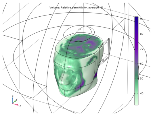
In the Settings window for 3D Plot Group, type Relative Permittivity, Average (emw) in the Label text field.
Volume 1
1
Right-click Relative Permittivity, Average (emw) and choose Volume.
2
In the Settings window for Volume, locate the Expression section.
3
In the Expression text field, type emw.epsrAv.
4
Locate the Coloring and Style section. From the Color table list, choose AuroraBorealis.
Selection 1
1
Right-click Volume 1 and choose Selection.
2
Filter 1
1
In the Model Builder window, right-click Volume 1 and choose Filter.
2
In the Settings window for Filter, locate the Element Selection section.
3
In the Logical expression for inclusion text field, type z<0.05.
4
In the Relative Permittivity, Average (emw) toolbar, click  Plot.
5
Click the  Zoom In button in the Graphics toolbar.
Average relative permittivity is visualized in Figure 1.