
|
|
|

|
1
|
|
2
|
Browse to the model’s Application Libraries folder and double-click the file porous_microchannel_heat_sink.mph.
|
|
1
|
|
2
|
|
1
|
In the Model Builder window, expand the Component 1 (comp1)>Definitions node, then click Variables 1.
|
|
2
|
|
1
|
|
2
|
|
3
|
Find the Studies subsection. In the Select Study tree, select Preset Studies for Selected Multiphysics>Stationary, One-Way NITF.
|
|
4
|
|
5
|
|
1
|
|
2
|
|
3
|
From the Method list, choose BOBYQA, because the BOBYQA solver is generally the fastest of the derivative-free solvers when the objective function is smooth. Reduce the Optimality tolerance to reduce the simulation time further.
|
|
4
|
|
5
|
|
6
|
|
7
|
|
1
|
|
2
|
|
4
|
|
1
|
|
2
|
|
3
|
|
4
|
|
1
|
|
2
|
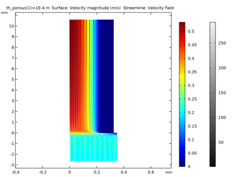
In the Settings window for 2D Plot Group, type Velocity, Cross Section, Optimization in the Label text field.
|
|
3
|
|
4
|
|
5
|
|
1
|
|
2
|
|
3
|
|
4
|
|
5
|
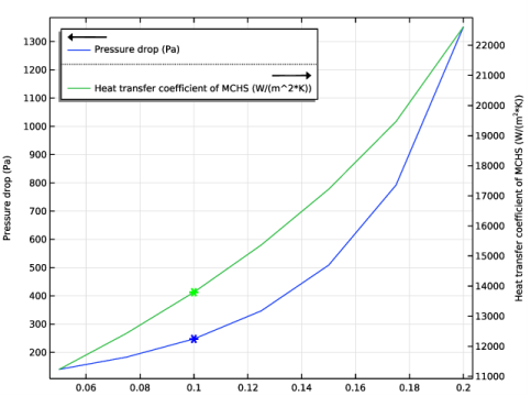
Locate the Expressions section. In the table, enter the following settings:
|
|
6
|
|
1
|
In the Model Builder window, right-click Heat-Transfer Coefficient and Pressure Drop and choose Table Graph.
|
|
2
|
|
3
|
|
4
|
|
5
|
|
6
|
Click to expand the Preprocessing section. Find the x-axis column subsection. From the Preprocessing list, choose Linear.
|
|
7
|
In the Scaling text field, type 1000. This is necessary because the porous layer thickness as control parameter of the optimization is saved in m whereas in the existing table it is plotted in mm.
|
|
8
|
Locate the Coloring and Style section. Find the Line markers subsection. From the Marker list, choose Asterisk.
|
|
9
|
|
1
|
|
2
|
|
3
|
|
4
|
|
5
|
|
6
|
|
1
|
|
2
|
|
3
|
|
4
|
|
5
|
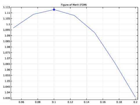
Click Replace Expression in the upper-right corner of the y-Axis Data section. From the menu, choose Component 1 (comp1)>Definitions>Variables>FOM - Figure of Merit.
|
|
6
|
|
7
|
|
8
|
|
9
|
|
10
|
|
1
|
|
2
|
|
3
|
|
4
|
|
5
|
|
6
|
|
7
|
Locate the Preprocessing section. Find the x-axis column subsection. From the Preprocessing list, choose Linear.
|
|
8
|
|
9
|
|
10
|
|
11
|
|
1
|
|
2
|
|
3
|
|
4
|
|
5
|