Performance of a Porous Microchannel Heat Sink

This model studies the performance of a microchannel heat sink (MCHS) with a porous block structure and compares its performance with that of a conventional MCHS. Todays demands on electronic components to become smaller and more efficient at the same time place equally high demands on the corresponding cooling devices. The use of porous material along the flow channels can enhance the heat transfer, by increasing the heat transfer surface area. At the same time, the pressure drop is also increased, requiring more pumping power. With a parametric study over the thickness of the porous substrate an optimized design of the porous MCHS can be found.

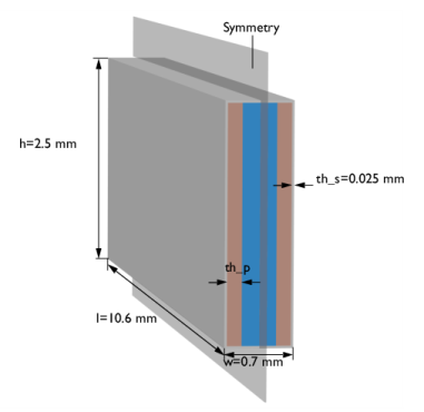
Figure 1: Geometry and operating conditions of the porous MCHS.

Model Definition

The design and operating conditions are taken from Ref. 1 and are illustrated in Figure 1. The problem can be reduced to modeling only one half of a single channel. This is sufficient, because the performance is mainly influenced by the pressure drop and heat transfer from the bottom boundary to the water in the channel. The geometry of the modeled domain is shown in Figure 2.

Figure 2: Geometry of the modeling domain. The free flow domain used to provide the inflow profile for the MCHS is not shown.

The flow channels contain sintered porous metal blocks with a porosity of ε = 0.402 on each side. A heat source with qin = 100 W/cm2 is attached to the bottom. Water with an inlet velocity of u = 0.2m/s and a temperature of Tin = 300 K is used as cooling fluid. The flow is assumed to be laminar, incompressible and stationary. The flow properties are also independent of the temperature field. Inside the porous domains the governing equation is the Brinkman equation with a Forchheimer correction term (also known as the Brinkman-Forchheimer or Darcy-Brinkman-Forchheimer equation). The pressure drop depends on the velocity field u as

(1)

where μ (Pa·s) is the fluid viscosity, ρ (kg/m3) the density, and κ (m2) the permeability of the porous substrate.

To evaluate the performance of the porous MCHS over the conventional MCHS, the first computation solves the model assuming only free flow. Then, a second study performs a parametric sweep over the thickness of the porous substrate (thp). The following performance parameters are evaluated:

Pressure drop, that is the pressure difference between inlet and outlet of the porous MCHS

Average heat transfer coefficient of the MCHS, given by

(2)

with the average wall temperature at the bottom centerline

Reynolds number is defined as

(3)

with the hydraulic diameter Dh (m) that is defined based on the length and width of the free flow channel, lf and wf respectively, as follows:

The Nusselt number describes the ratio of convective to conductive heat transfer according to

(4)

where kf is the fluids thermal conductivity.

The Figure of Merit (FOM) compares the performance of two different designs with the following expression:

(5)

The index base refers to the values for the MCHS without the porous structure and Ω = uinlfwfΔp is the pumping power.

Equation 1 is valid for 1 ≤ Re ≤ 1000. An estimation of the Reynolds number (Equation 3) results in Re ∼ 300 such that the choice of the Brinkman-Forchheimer equation is valid.

Results and Discussion

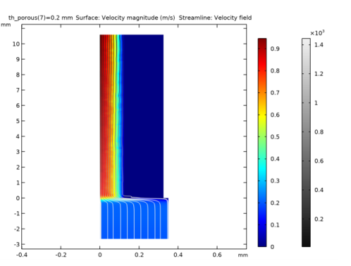
Figure 3 shows the velocity field in a cross section of the channel. The velocity magnitude inside the porous structure is small (dark blue) compared to that of the free flow channel.

Figure 3: Cross section of the velocity field along the channel (scaled view). The dark blue color indicates the porous structure, because the velocity magnitude is small in this area.

The temperature distribution is shown together with the velocity profile in Figure 4.

Figure 4: Temperature distribution (color) and velocity field (arrows) with the gray scale indicating the pressure.

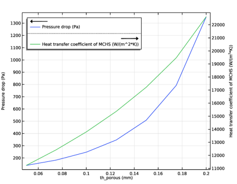
The pressure drop and average heat transfer coefficient as a function of the thickness of the porous structure are shown in Figure 5. With increasing thickness, both values also increase.

Figure 5: Pressure drop and average heat transfer coefficient.

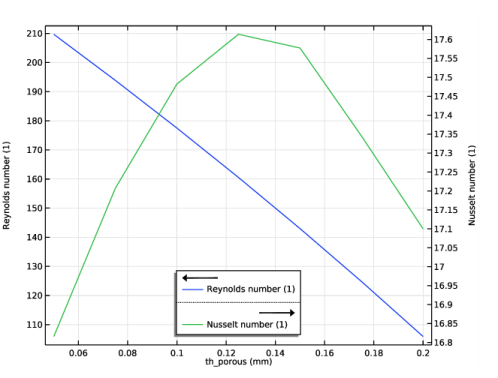
Figure 6 shows how the dimensionless Reynolds and Nusselt numbers depend on this thickness. The Reynolds number decreases with increasing thp and varies in the range from 100 to 210, meaning that the choice of the Brinkman-Forchheimer equation is justified. The Nusselt number has a maximum at thp = 0.125 mm.

Figure 6: Reynolds and Nusselt numbers.

The Figure of Merit (Figure 7) shows that the optimal performance is achieved for thp = 0.1 mm.

Figure 7: The Figure of Merit comparing the performances of the porous and the conventional MCHS.

Notes About the COMSOL Implementation

This model shows how to analyze the performance of the porous MCHS for varying porous substrate thickness. The model geometry and operating conditions are fully parametrized, such that you can easily extend the model for various parameters, as for example the inlet velocity or other channel dimensions.

Reference

1. A. Ghahremannezhad and K. Vafai, “Thermal and hydraulic performance enhancement of microchannel heat sinks utilizing porous substrates,” Int. J. Heat Mass Transfer, vol. 122, pp. 1313–1326, 2018.

Porous_Media_Flow_Module/Heat_Transfer/porous_microchannel_heat_sink

Modeling Instructions

Root

Start by loading the model file that contains the geometry and selections used throughout the modeling process.

From the menu, choose .

Browse to the model’s Application Libraries folder and double-click the file porous_microchannel_heat_sink_geom_sequence.mph.

Global Definitions

Parameters 1

The geometry parameters are already present after loading the file. Add a few more parameters for the material properties and operating conditions.

In the window, under click .

In the window for , locate the section.

In the table, enter the following settings:


Name	Expression	Value	Description
rho_f	998[kg/m^3]	998 kg/m³	Density, fluid
mu_f	8.55e-4[Pa*s]	8.55E-4 Pa·s	Viscosity, fluid
k_f	0.6[W/(m*K)]	0.6 W/(m·K)	Thermal conductivity, fluid
Cp_f	4182[J/(kg*K)]	4182 J/(kg·K)	Heat capacity, fluid
por	0.404	0.404	Porosity
d_p	20[um]	2E-5 m	Pore size
kappa	d_p^2/150*por^3/(1-por)^2	4.9502E-13 m²	Permeability
q_in	50[W/cm^2]	5E5 W/m²	Heat load
T_in	300[K]	300 K	Inlet temperature
u_in	0.2[m/s]	0.2 m/s	Inlet velocity

Add Physics

In the toolbar, click

to open the window.

Go to the window.

In the tree, select .

Click in the window toolbar.

In the tree, select .

Click in the window toolbar.

In the toolbar, click

to close the window.

Add Multiphysics

In the toolbar, click

to open the window.

Go to the window.

In the tree, select .

Click in the window toolbar.

In the toolbar, click

to close the window.

This adds the coupling between the and interfaces.

Next, add the materials. For the fluid use a user-defined material with the parameters defined above. Load steel from the Material Library.

Global Definitions

Water

In the window, under right-click and choose .

In the window for , type Water in the text field.

Add Material

In the toolbar, click

to open the window.

Go to the window.

In the tree, select .

Click in the window toolbar.

In the toolbar, click

to close the window.

Materials

Material Link 1 (matlnk1)

In the window, under right-click and choose .

Material Link 2 (matlnk2)

Right-click and choose .

In the window for , locate the section.

From the list, choose .

Locate the section. From the list, choose .

Porous Material 1 (poromat1)

Right-click and choose .

In the window for , locate the section.

From the list, choose .

Locate the section. From the list, choose .

Fluid 1 (poromat1.fluid1)

Right-click and choose .

Solid 1 (poromat1.solid1)

In the window, right-click and choose .

In the window for , locate the section.

From the list, choose .

In the θs text field, type 1-por.

Now, set up the domain conditions. This determines which material properties are required and you can fill in the missing materials afterward. For this step the selections are helpful.

Laminar Flow (spf)

Assume incompressible flow.

In the window, under click .

In the window for , locate the section.

From the list, choose .

Select the check box.

Locate the section. From the list, choose .

Fluid and Matrix Properties 1

In the toolbar, click

and choose .

In the window for , locate the section.

From the list, choose .

Locate the section. From the list, choose .

From the εp list, choose . In the associated text field, type por.

From the list, choose .

From the κ list, choose . In the associated text field, type kappa.

Heat Transfer in Solids and Fluids (ht)

Fluid 1

In the window, under click .

In the window for , locate the section.

From the list, choose .

Porous Medium 1

In the toolbar, click

and choose .

In the window for , locate the section.

From the list, choose .

Porous Matrix 1

In the window, expand the node, then click .

In the window for , locate the section.

From the list, choose .

You can now specify the values of the missing material properties.

Global Definitions

Water (mat1)

In the window, under click .

In the window for , locate the section.

In the table, enter the following settings:


Property	Variable	Value	Unit	Property group
Density	rho	rho_f	kg/m³	Basic
Dynamic viscosity	mu	mu_f	Pa·s	Basic
Thermal conductivity	k_iso ; kii = k_iso, kij = 0	k_f	W/(m·K)	Basic
Heat capacity at constant pressure	Cp	Cp_f	J/(kg·K)	Basic
Ratio of specific heats	gamma	1	1	Basic

Complete the physics setup by adding the boundary conditions.

Laminar Flow (spf)

In the window, under click .

Inlet 1

In the toolbar, click

and choose .

In the window for , locate the section.

From the list, choose .

Locate the section. In the U0 text field, type u_in.

Outlet 1

In the toolbar, click

and choose .

In the window for , locate the section.

From the list, choose .

Symmetry 1

In the toolbar, click

and choose .

In the window for , locate the section.

From the list, choose .

Heat Transfer in Solids and Fluids (ht)

In the window, under click .

Boundary Heat Source 1

In the toolbar, click

and choose .

Select Boundary 7 only.

In the window for , locate the section.

In the Qb text field, type q_in.

Inflow 1

In the toolbar, click

and choose .

In the window for , locate the section.

From the list, choose .

Locate the section. In the Tustr text field, type T_in.

Outflow 1

In the toolbar, click

and choose .

In the window for , locate the section.

From the list, choose .

Symmetry 1

In the toolbar, click

and choose .

In the window for , locate the section.

From the list, choose .

To evaluate the performance, define new variables (see Equation 2 to Equation 5).

To evaluate the pressure drop define a nonlocal average coupling at the inlet of the porous MCHS. Use the average temperature of the centerline at the bottom surface to evaluate the heat transfer coefficient.

Definitions (comp1)

Average: Inlet of Porous MCHS

In the toolbar, click

and choose .

In the window for , locate the section.

From the list, choose .

Click the

button in the toolbar.

Select Boundaries 9 and 17 only.

In the text field, type Average: Inlet of Porous MCHS.

Average: Centerline, Bottom Surface

In the toolbar, click

and choose .

In the window for , locate the section.

From the list, choose .

Select Edge 7 only.

In the text field, type Average: Centerline, Bottom Surface.

Variables 1

In the window, right-click and choose .

In the window for , locate the section.

In the table, enter the following settings:


Name	Expression	Unit	Description
Dh	2width_channelheight_channel/(width_channel+height_channel)	m	Hydraulic diameter
dp	aveop1(p)	Pa	Pressure drop
Tw	aveop2(T)	K	Average wall temperature
Omega	spf.out1.Mflow/rho_f*dp	W	Pumping power
h_mchs	q_in/(Tw-T_in)	W/(m²·K)	Heat transfer coefficient of MCHS
Nu	h_mchs*Dh/k_f		Nusselt number
Re	rho_fu_inDh/mu_f		Reynolds number