Analyzing Porous Structures on the Microscopic Scale

Modeling flow through realistic porous structures is difficult due to the complexity of the structure itself. Resolving the flow field in detail is not feasible in real-life applications. Therefore, macroscopic approaches utilizing averaged quantities of the porous structure, such as porosity and permeability, are used. This example analyzes the flow field at the pore scale in detail. The results are used to validate and adapt the macroscopic description, which in turn are used to model large-scale porous geometries.

Model Definition

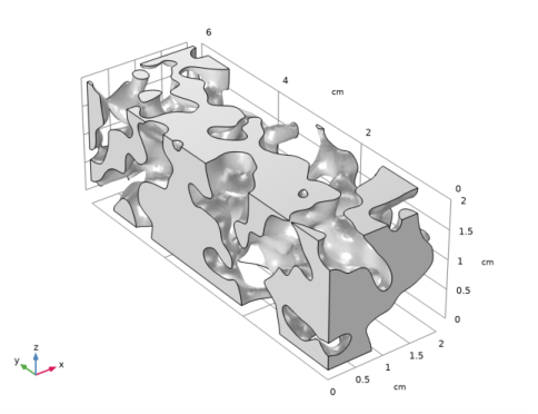
The modeled geometry shown in Figure 1 is a representative elementary volume (REV) whose properties are representative for the entire system.

Figure 1: Geometry of the REV’s pore volume.

Because only the area of the pore space is required for modeling, the porous matrix is not resolved explicitly. The REV has a quadratic cross section of 2 cm side length and a width of 6 cm. Water flows with a velocity of u = 0.1 mm/s and can flow out freely in the normal direction at the other end. The other boundaries are assumed to be symmetry boundaries. This does not correspond to the actual situation, but for modeling an REV, symmetry boundary conditions are very well suited.

To characterize the flow inside the porous structure one can estimate the Reynolds number according to

with the water density ρ = 1000 kg/m3 and viscosity μ = 10-3 Pa·s. The cross-section side length serves as the characteristic length scale, L. This results in Re = 2 and the Stokes equation can be used to describe the flow where inertia terms are neglected.

Finally, the goal of the model is to obtain the averaged values for porosity and permeability to describe a macroscopic model with, for example, Darcy’s law or the Brinkman equation. The porosity is defined as the fraction of pore space volume Vfluid to total volume Vtot:

To calculate the permeability κ (m2) the following relationship is used:

Approximating the pressure gradient ∇p by the pressure difference between the inlet and the outlet, Δp, divided by the side length L, and replacing the velocity vector u by the outlet velocity uout in the flow direction gives the expression

Results and Discussion

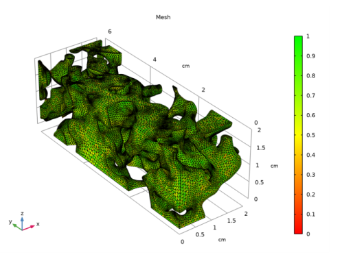
First of all it is interesting to have a look at the mesh, or rather the mesh quality. Although the mesh quality in itself says nothing about the quality of the results, a good mesh quality is beneficial for convergence. The overall mesh quality as shown in Figure 2 is very good.

Figure 2: Mesh quality plot.

The velocity field in the REV is shown in Figure 3. Characteristic for the flow in a porous material are areas with high and areas with low velocity. In some areas the flow also stagnates. This behavior is characterized by the permeability.

Figure 3: Velocity in the REV.

From the simulation the values for the porosity and permeability are obtained, with ε = 0.373 and

Notes About the COMSOL Implementation

The geometry is characterized by narrow regions and a complex free surface. This has a great influence on the mesh. The automatic meshing algorithm can be tuned by certain manual settings, which is beneficial for both mesh quality and performance.

Porous_Media_Flow_Module/Fluid_Flow/pore_scale_flow_3d

Modeling Instructions

From the menu, choose .

New

In the window, click

Model Wizard

In the window, click

In the tree, select .

Click .

Click

In the tree, select .

Click

Geometry 1

In the window, under click .

In the window for , locate the section.

From the list, choose .

Import 1 (imp1)

In the toolbar, click

In the window for , locate the section.

Click .

Browse to the model’s Application Libraries folder and double-click the file pore_scale_flow_3d.mphbin.

Click .

Global Definitions

Add some parameters that are used to set up the model.

Parameters 1

In the window, under click .

In the window for , locate the section.

In the table, enter the following settings:


Name	Expression	Value	Description
rho_f	1000[kg/m^3]	1000 kg/m³	Fluid density
mu_f	1e-3[Pa*s]	0.001 Pa·s	Fluid viscosity
u_in	1e-4[m/s]	1E-4 m/s	Inlet velocity
width	2[cm]	0.02 m	REV width
length	6[cm]	0.06 m	REV length
V_tot	width^2*length	2.4E-5 m³	Total REV volume

Materials

Water

In the window, under right-click and choose .

In the window for , type Water in the text field.

Locate the section. In the table, enter the following settings:


Property	Variable	Value	Unit	Property group
Density	rho	rho_f	kg/m³	Basic
Dynamic viscosity	mu	mu_f	Pa·s	Basic

Creeping Flow (spf)

In the window, under click .

In the window for , click to expand the section.

From the list, choose .

Linear elements reduce the number of degrees of freedom to be solved. Because the geometry already requires a fine mesh, using linear elements decreases computational time and memory requirements while maintaining sufficient accuracy.

Inlet 1

In the toolbar, click

and choose .

Select Boundary 2 only.

In the window for , locate the section.

In the U0 text field, type u_in.

Locate the section. Click

In the dialog box, type Inlet in the text field.

Click .

Outlet 1

In the toolbar, click

and choose .

Select Boundaries 16 and 22 only.

In the window for , locate the section.

Select the check box.

Locate the section. Click

In the dialog box, type Outlet in the text field.

Click .

Create a few more selections to use them throughout the model set up.

Definitions

In the window, expand the node.

Wall

In the window, expand the node.

Right-click and choose .

In the window for , type Wall in the text field.

Locate the section. From the list, choose .

Select Boundaries 4, 10, and 30 only.

It might be easier to select the correct boundary by using the window. To open this window, in the toolbar click and choose . (If you are running the cross-platform desktop, you find in the main menu.)

All boundaries

In the toolbar, click

In the window for , locate the section.

From the list, choose .

Select the check box.

In the text field, type All boundaries.

Symmetry

In the toolbar, click

In the window for , type Symmetry in the text field.

Locate the section. From the list, choose .

Locate the section. Under , click

In the dialog box, select in the list.

Click .

In the window for , locate the section.

Under , click

In the dialog box, in the list, choose , , and .

Click .

Creeping Flow (spf)

Symmetry 1

In the toolbar, click

and choose .

In the window for , locate the section.

From the list, choose .

Mesh 1

The physics-controlled mesh is a good starting point. Modify the sequence to help the meshing algorithm and improve overall quality.

In the window, under click .

In the window for , locate the section.

From the list, choose .

Locate the section. From the list, choose .

Size

In the window, under click .

In the window for , click to expand the section.

Locate the section. Click the button.

Locate the section. In the text field, type 0.125.

Size 1

In the window, click .

In the window for , locate the section.

Click the button.

Locate the section. Select the check box.

In the associated text field, type 0.06.

Corner Refinement 1

In the window, right-click and choose .

In the window for , click

Corner refinement will not improve the mesh significantly, hence it is disabled.

Free Triangular 1

In the toolbar, click

and choose .

In the window for , locate the section.

From the list, choose .

Click

Creating a surface mesh for the freeform surface first, helps the meshing algorithm.

To ensure a good quality of the mesh, we use the following settings for the tetrahedral mesh.

Free Tetrahedral 1

In the window, click .

In the window for , click to expand the section.

Select the check box.

From the list, choose .

Click

In the toolbar, click

Results

Mesh 1

Compare with Figure 2. The overall mesh quality is very good. The amount of low quality mesh elements (skewness) is low. Mesh quality is not an indication for the accuracy of the solution, but it affects the convergence behavior.

Study 1

In the window, click .

In the window for , locate the section.

Clear the check box.

In the toolbar, click

Create the plot as shown in Figure 3.

In the toolbar, click

and choose .

Results

Surface 1

In the window for , locate the section.

From the list, choose .

Velocity

In the toolbar, click

In the window for , type Velocity in the text field.

Locate the section. Clear the check box.

Surface 1

Right-click and choose .

In the window for , locate the section.

From the list, choose .

Locate the section. In the text field, type 1.

Locate the section. From the list, choose .

From the list, choose .

Line 1

In the window, right-click and choose .

In the window for , locate the section.

From the list, choose .

Locate the section. From the list, choose .

From the list, choose .

In the toolbar, click

From the list, choose . Choose a darker shade of gray.

Streamline 1

Right-click and choose .

In the window for , locate the section.

From the list, choose .

Locate the section. In the text field, type 40.

Locate the section. Find the subsection. From the list, choose .

Select the check box.

In the associated text field, type 0.0075.

Color Expression 1

Right-click and choose .

In the window for , locate the section.

From the list, choose .

Next, determine the porosity and permeability for our REV in order to perform simulations at the macroscopic level.

Definitions

Integration 1 (intop1)

In the toolbar, click

and choose .

In the window for , locate the section.

From the list, choose .

Average Inlet

In the toolbar, click

and choose .

In the window for , locate the section.

From the list, choose .

In the text field, type Average Inlet.

Average Outlet

In the toolbar, click

and choose .

In the window for , locate the section.

From the list, choose .

In the text field, type Average Outlet.

Variables 1

In the window, right-click and choose .

In the window for , locate the section.

In the table, enter the following settings:


Name	Expression	Unit	Description
por	intop1(1)/V_tot		Porosity
dPdL	-(aveop2(p)-aveop1(p))/length	N/m³	Pressure drop
u_out	spf.out1.massFlowRate/rho_f/width^2	m/s	Superficial outlet velocity
kappa	u_out*mu_f/dPdL	m²	Permeability

Since you have introduced new variables, the solution needs to be updated. It is not necessary to compute the study again.

Study 1

In the toolbar, click

Results

Global Evaluation 1

In the toolbar, click

In the window for , click in the upper-right corner of the section. From the menu, choose .

Click in the upper-right corner of the section. From the menu, choose .

Click

The results are shown in the window. The porosity is 0.373 and the permeability is about 3e-8m2. These results can now be used for calculations of large scale models.

Streamline 1

To make the results even more descriptive, create an animation.

In the window, click .

In the window for , locate the section.

Find the subsection. From the list, choose .

In the text field, type 2000.

Animation 1

In the toolbar, click

and choose .

You can adjust the number of frames to obtain a smooth animation of the interactive arrows. This animation visualizes very nicely that there are regions in the porous medium with both very slow and very high velocity.