Geothermal Heating from a Pond Loop

Ponds and lakes can serve as thermal reservoirs in geothermal heating applications. In this example, fluid circulates underwater through polyethylene piping in a closed system. The pipes are coiled in a slinky shape and mounted onto sleds. The Nonisothermal Pipe Flow interface sets up and solves the equations for the temperature and fluid flow in the pipe system, where the geometry is represented by lines in 3D.

Figure 1: A sled carrying pipe coils shown before the system is submerged.

Model Definition

Geometry

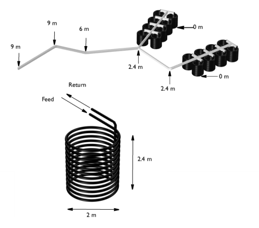
High density polyethylene pipe (20 mm diameter) is rolled into sixteen coils. Groups of eight coils are mounted on two sleds. Each coil has a radius of 1 m and a length of approximately 75 m. The coil groups are connected to feed and return piping with a diameter of 50 mm (see Figure 2). The coil groups are 2.4 m in height an sit at the bottom of a pond that is 6 m deep. The total length of the piping is 1446 m.

Figure 2: Polyethylene pipe system. Elevation above the pond bottom is indicated. Feed and return piping (gray) is 50 mm in diameter while coils (black) are 20 mm in diameter. The pipes are insulated above the pond surface.

The heat exchange between pond water and pipe fluid depends on the temperature difference between the two. A slow current in the pond makes the heat transfer more effective than water at rest. The pond is warmer closer to the surface, as shown by the temperature data in Table 1 below.

Table 1: Pond Temperature.
Elevation (m)	Temperature (K)
0	284
2	288
4	291
6	293

It is easy to set up a function in the software with linear interpolation between points so that the varying pond temperature can be taken into account in the simulation.

Flow Equations

The continuity and momentum equations below describe the stationary flow inside the pipe system:

(1)

Above, A (SI unit: m2) is the cross section area of the pipe, ρ (SI unit: kg/m3) is the density, u (SI unit: m/s) is the fluid velocity, and p (SI unit: N/m2) is the pressure and F (SI unit: N/m3) is a volume force, like gravity.

Gravity can be included explicitly in the model, but since the variation in density is negligible, and the model is not pressure driven, the only effect of including gravity is a change in the total pressure level. It is therefore common modeling practice to exclude gravity by setting F=0 and interpret the pressure variable as the reduced pressure

, where z0 is the datum level of the free liquid surface. This reduces the model complexity and yields the same results.

Expressions for the Darcy Friction Factor

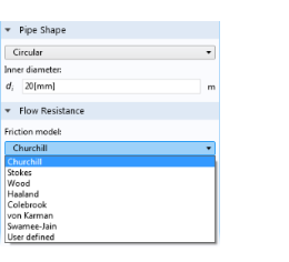
The right-hand side of Equation 1 describes the pressure drop due to internal viscous shear. The term contains the Darcy friction factor, fD, which is a function of the Reynolds number and the surface roughness divided by the hydraulic pipe diameter, e/dh. The Nonisothermal Pipe Flow interface provides a library of built-in expressions for the Darcy friction factor, fD.

Figure 3: Select from different predefined Friction models in the Pipe Properties node.

This example uses the Churchill relation (Ref. 1) that is valid for laminar flow, turbulent flow, and the transitional region in between. The Churchill relation is:

(2)

where

As seen from the equations above, the friction factor is a function of the surface roughness divided by diameter of the pipe. Surface roughness data can be selected from a predefined list in the Pipe Properties feature.

The Churchill equation is also a function of the fluid properties, through the Reynolds number:

The physical properties of water as function of temperature are directly available from the software’s built-in material library. Inspection of Equation 2 reveals that for low Reynold’s number (at laminar flow), the friction factor is 64/Re, and for very high Reynolds number, the friction factor is independent of Re.

Heat Transfer Equations

The energy equation for the pipeline flow is:

(3)

where Cp (SI unit: J/(kg·K)) is the heat capacity at constant pressure, T is the temperature (SI unit: K), and k (SI unit: W/(m·K)) is the thermal conductivity. The second term on the right-hand side of Equation 3 corresponds to friction heat dissipated due viscous shear. Qwall (SI unit: W/m) is a source/sink term due to heat exchange with the surroundings through the pipe wall:

(4)

Where Z (m) is the wetted perimeter of the pipe, h (W/(m2·K)) an overall heat transfer coefficient and Text (K) the external temperature outside of the pipe.

The overall heat transfer coefficient includes contribution from internal film resistance, wall resistance, and external film resistance.

Figure 4: Temperature distribution across the pipe wall.

For a circular pipe, under assumption that the heat transfer through the wall is quasi static and that the temperature is equal around the circumference of the pipe, an effective hZ in Equation 4 is given by

.where rn is the outer radius of wall n, hint and hext are the film heat transfer coefficients on the inside and outside of the tube, and kn is the thermal conductivity of wall n.

The film resistance inside the pipe is given by:

The internal Nusselt number is taken as 3.66 for the laminar flow regime (Ref. 2), and for the turbulent flow regime the Gnielinski correlation for internal pipe flow is used (Ref. 3):

The external film resistance around the pipe is:

A slow current is present in the pond. For external forced convection around a pipe, COMSOL uses the Churchill and Bernstein (Ref. 4) relation for Nu, valid for all Re and for Pr > 0.2,:

where Pr = Cpμ/k.

Properties of the pipe wall is given in the table below.

Table 2: Pipe properties.
Name	Value	Description
dwall	2 mm	Pipe wall thickness
kwall	0.46 W/(m·K)	Pipe wall thermal conductivity

Results and Discussion

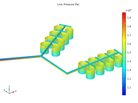
Figure 5 shows the pressure (Pa) in the 1446 m pipe system assuming that water enters the system at a rate of 4 l/s.

Figure 5: Pressure drop over the pipe system.

The plot below shows the temperature (K) distribution for the pipe fluid. It enters the pipe system at 5 °C and exits with a temperature of approximately 11 °C.

Figure 6: Temperature of the pipe fluid.

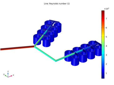
Turbulent flow conditions in the loop are important for good heat exchange between the pipes and the surroundings. A plot of the Reynolds number is shown in Figure 7, confirming that flow is turbulent (Re > 3000) throughout the system.

Figure 7: The Reynolds number in the pipe loop confirms that the flow conditions are turbulent.

This model is also available in an extended version in the Introduction to Pipe Flow Module booklet.

References

1. S.W. Churchill, “Friction factor equation spans all fluid-flow regimes,” Chem. Eng., vol. 84, no. 24, p. 91, 1997.

2. F.P. Incropera and D.P. DeWitt, Fundamentals of Heat and Mass Transfer, 4th ed., John Wiley & Sons, 1996. Eq 8.62 and Eq 9.34, respectively.

3. V. Gnielinski, “New Equation for Heat and Mass Transfer in Turbulent Pipe and Channel Flow,” Int. Chem. Eng., vol. 16, pp. 359–368, 1976.

4. S.W. Churchill and M. Bernstein, “A Correlating Equation for Forced Convection from Gases and Liquids to a Circular Cylinder in Crossflow,” J Heat Transfer, vol. 99, p. 300, 1977.

Pipe_Flow_Module/Heat_Transfer/geothermal_heating

Modeling Instructions

From the menu, choose .

New

In the window, click

Model Wizard

In the window, click

In the tree, select .

Click .

Click

In the tree, select .

Click

Geometry 1

Start by creating the piping system geometry. You can simplify this by inserting a prepared geometry sequence from file:

In the toolbar, click

Browse to the model’s Application Libraries folder and double-click the file geothermal_heating_geom_sequence.mph.

In the toolbar, click

The complete instructions for creating this geometry can be found in the appendix at the end of this document.

Definitions

Now add some external data in the form of interpolation tables and variables.

Interpolation 1 (int1)

In the toolbar, click

and choose .

In the window for , locate the section.

In the table, enter the following settings:


t	f(t)
0	284
2	288
4	291
6	293

Locate the section. In the text field, type m.

In the text field, type K.

Variables 1

In the toolbar, click

and choose .

In the window for , locate the section.

Click

Browse to the model’s Application Libraries folder and double-click the file geothermal_heating_variables.txt.

Add Material

In the toolbar, click

to open the window.

Go to the window.

In the tree, select .

Click in the window toolbar.

In the toolbar, click

to close the window.

Nonisothermal Pipe Flow (nipfl)

Pipe Properties 1

In the window, under click .

In the window for , locate the section.

From the list, choose .

In the di text field, type 20[mm].

Temperature 1

In the window, click .

In the window for , locate the section.

In the Tin text field, type 5[degC].

Pipe Properties 2

In the toolbar, click

and choose .

Select Edges 1–12, 15, 17–21, 27–29, 33–35, 39, 41–45, 51–53, 57–59, 63, 65–69, 75–77, 81–83, 87, 89–91, 97, 98, 102, and 103 only.

To make the selection easily, first click and then click . In the window, draw a box around the pipes to select them. Click the button. Alternatively, copy the entity numbers from the text, click in the selection box, and then press Ctrl+V.