
|
|
|

|
1
|
|
2
|
|
3
|
Click Add.
|
|
4
|
Click
|
|
5
|
|
6
|
Click
|
|
1
|
|
2
|
|
1
|
|
2
|
|
3
|
|
1
|
|
2
|
|
3
|
|
1
|
|
2
|
|
3
|
|
1
|
|
2
|
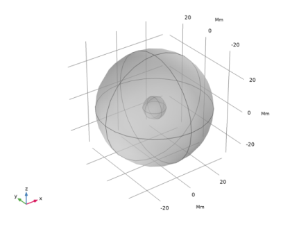
Select the object sph2 only.
|
|
3
|
|
4
|
|
5
|
|
6
|
Select the object sph1 only.
|
|
7
|
|
8
|
|
9
|
|
1
|
|
2
|
|
3
|
|
4
|
|
5
|
On the object dif1, select Boundaries 1–4, 9, 10, 13, and 16 only.
|
|
1
|
|
2
|
|
3
|
|
4
|
|
1
|
|
2
|
In the Settings window for Charged Particle Tracing, locate the Particle Release and Propagation section.
|
|
3
|
|
4
|
|
1
|
In the Model Builder window, under Component 1 (comp1)>Charged Particle Tracing (cpt) click Particle Properties 1.
|
|
2
|
|
3
|
|
1
|
|
2
|
|
3
|
|
4
|
|
1
|
|
2
|
|
3
|
|
4
|
Locate the Initial Velocity section. From the Initial velocity list, choose Kinetic energy and direction.
|
|
5
|
|
6
|
|
1
|
|
2
|
In the Settings window for Auxiliary Dependent Variable, locate the Auxiliary Dependent Variable section.
|
|
3
|
|
1
|
|
2
|
In the Settings window for Auxiliary Dependent Variable, locate the Auxiliary Dependent Variable section.
|
|
3
|
|
1
|
|
3
|
|
4
|
|
5
|
|
6
|
Click to expand the New Value of Auxiliary Dependent Variables section. Select the Assign new value to auxiliary variable : Lm check box.
|
|
7
|
|
1
|
In the Model Builder window, under Component 1 (comp1)>Charged Particle Tracing (cpt) right-click Release from Grid 1 and choose Duplicate.
|
|
2
|
|
3
|
|
4
|
Locate the Initial Value of Auxiliary Dependent Variables section. From the Distribution function list, choose List of values.
|
|
5
|
Click
|
|
6
|
|
7
|
|
8
|
|
9
|
Click Replace.
|
|
10
|
In the Settings window for Release from Grid, locate the Initial Value of Auxiliary Dependent Variables section.
|
|
11
|
Select the second Initialize before particle momentum check box, which corresponds to the variable for equatorial pitch angle Ea.
|
|
1
|
|
2
|
|
3
|
|
4
|
In the Physics and variables selection tree, select Component 1 (comp1)>Charged Particle Tracing (cpt)>Auxiliary Dependent Variable 1.
|
|
5
|
Click
|
|
6
|
In the Physics and variables selection tree, select Component 1 (comp1)>Charged Particle Tracing (cpt)>Auxiliary Dependent Variable 2.
|
|
7
|
Click
|
|
8
|
In the Physics and variables selection tree, select Component 1 (comp1)>Charged Particle Tracing (cpt)>Velocity Reinitialization 1.
|
|
9
|
Click
|
|
10
|
In the Physics and variables selection tree, select Component 1 (comp1)>Charged Particle Tracing (cpt)>Release from Grid 2.
|
|
11
|
Click
|
|
12
|
|
13
|
|
14
|
|
15
|
Click Replace.
|
|
16
|
|
1
|
|
2
|
|
1
|
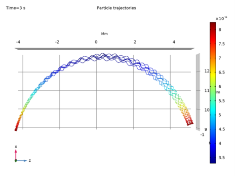
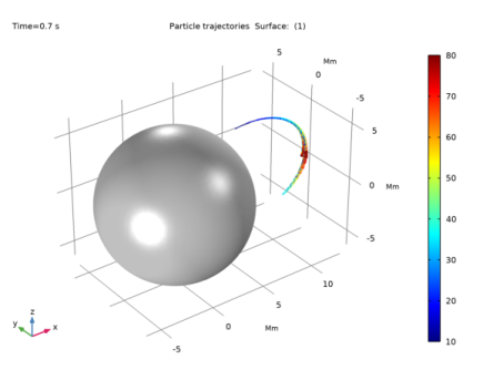
In the Model Builder window, expand the Particle Trajectories (cpt) node, then click Particle Trajectories 1.
|
|
2
|
|
3
|
|
4
|
|
6
|
|
7
|
|
8
|
|
1
|
In the Model Builder window, expand the Particle Trajectories 1 node, then click Color Expression 1.
|
|
2
|
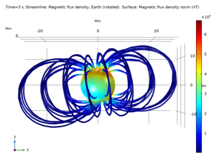
In the Settings window for Color Expression, click Replace Expression in the upper-right corner of the Expression section. From the menu, choose Component 1 (comp1)>Charged Particle Tracing>Fields>cpt.mf1.normB - Magnetic flux density norm - T.
|
|
3
|
|
1
|
|
2
|
|
3
|
|
1
|
|
2
|
|
3
|
|
4
|
|
1
|
|
2
|
|
3
|
|
1
|
|
2
|
In the Settings window for Streamline, click Replace Expression in the upper-right corner of the Expression section. From the menu, choose Component 1 (comp1)>Charged Particle Tracing>Fields>cpt.mf1.Berx,...,cpt.mf1.Berz - Magnetic flux density, Earth (rotated).
|
|
3
|
Locate the Streamline Positioning section. From the Positioning list, choose Starting-point controlled.
|
|
4
|
|
5
|
|
6
|
Locate the Coloring and Style section. Find the Line style subsection. From the Type list, choose Tube.
|
|
1
|
|
2
|
In the Settings window for Color Expression, click Replace Expression in the upper-right corner of the Expression section. From the menu, choose Component 1 (comp1)>Charged Particle Tracing>Fields>cpt.mf1.normB - Magnetic flux density norm - T.
|
|
3
|
|
1
|
|
2
|
|
3
|
|
4
|
Click Replace Expression in the upper-right corner of the Expression section. From the menu, choose Component 1 (comp1)>Charged Particle Tracing>Fields>cpt.mf1.normB - Magnetic flux density norm - T.
|
|
5
|
|
6
|
|
7
|
|
1
|
|
2
|
|
3
|
|
1
|
|
2
|
|
3
|
|
1
|
|
2
|
|
3
|
|
4
|
|
5
|
|
1
|
|
2
|
|
3
|
In the Physics and variables selection tree, select Component 1 (comp1)>Charged Particle Tracing (cpt)>Release from Grid 1.
|
|
4
|
Click
|
|
5
|
|
6
|
|
7
|
|
8
|
Click Replace.
|
|
9
|
|
1
|
|
2
|
|
1
|
In the Model Builder window, expand the Particle Trajectories (cpt) 1 node, then click Particle Trajectories 1.
|
|
2
|
|
3
|
|
4
|
|
1
|
In the Model Builder window, expand the Particle Trajectories 1 node, then click Color Expression 1.
|
|
2
|
|
3
|
|
1
|
|
2
|
|
3
|
|
4
|
|
5
|
|
6
|
|
7
|
|
1
|
|
2
|
|
3
|
|
4
|
|
5
|
|
6
|
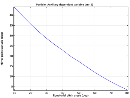
In the associated text field, type Equatorial pitch angle (deg).
|
|
7
|
|
8
|
In the associated text field, type Mirror point latitude (deg).
|
|
1
|
|
2
|
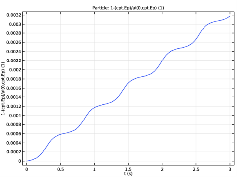
In the Settings window for Particle, click Replace Expression in the upper-right corner of the y-Axis Data section. From the menu, choose Component 1 (comp1)>Charged Particle Tracing>Auxiliary dependent variables>Lm - Auxiliary dependent variable Lm.
|
|
3
|
|
4
|
|
5
|