Child’s Law Benchmark

Space charge limited emission is a phenomenon that restricts the number of electrons or other charged particles that can be released from a surface. As the current of electrons released by a cathode increases, so does the charge density in the immediate vicinity of the cathode. This distribution of charge density exerts an electric force on the emitted electrons, directed toward the cathode. The space charge limited current is the maximum current that can be released such that the emitted particles are not repelled back toward the cathode.

In this example, the space charge limited current in a plane-parallel vacuum diode is computed using the dedicated particle release feature. A bidirectional coupling is set up in which the electrons produce a distribution of space charge density that contributes to the electric potential being solved for. The resulting electric potential distribution and current are compared with the analytical solution given by Child’s law.

The Application Library example Thermionic Emission in a Planar Diode expands upon this example by employing the more detailed Langmuir-Fry model, in which the initial thermal distribution of electron velocity at the cathode is also taken into account.

Model Definition

The model geometry is two-dimensional but can be thought of as quasi-1D because the current and electric potential are uniform in the y-direction. Electrons are emitted from a grounded cathode located at position x = 0 and propagate toward an extraction grid at a fixed potential V0 (SI unit: V) located at x = d, where d > 0. Space charge limited emission occurs when any further increase in current would repel electrons back toward the cathode; this is equivalent to enforcing the boundary condition

on the cathode surface, in addition to the usual boundary condition

for a grounded surface.

Ensuring Numerical Convergence

The space charge limited current is computed using an iterative process in which the particle trajectories and electric potential are computed in alternating steps. The values of variables not solved for in one step are always taken from the most recent iteration of the other. In this way, successively better approximations of the current can be computed. However, if the space charge limited current is significantly overestimated during any iteration, then all of the electrons would immediately be repelled back toward the cathode and the charge density would become saturated in the mesh elements adjacent to the cathode, causing the model to fail. To avoid this overestimation of the space charge limited current, only a small fraction of the space charge density is used to calculate the electric potential during early iterations. This fraction of the space charge density is gradually increased until it reaches unity in the specified in the Settings window for the node.

To further improve the stability and robustness of the model, the electrons are not released precisely at the cathode, but rather a short distance away from it where the gradient of the electric potential is slightly greater than zero. To do so, the feature is applied to the boundary at x = 0. Instead of representing the cathode, the left side of the geometry represents an emission surface a short distance dbuf away from the cathode. The electric potential is computed in the narrow region between the cathode and the emission surface, allowing the initial particle velocity at the emission surface to be defined. The electric potential to the right of the emission surface can then be computed using the space charge density computed by the node.

The study step sets up a solver loop in which the particle trajectories are computed using a time-dependent solver, while the electric potential is computed using a stationary solver. The solver sequence alternates between these two solvers for a specified number of iterations, always using the previous solution for the variables not solved for. In this way, a self-consistent solution, in which the particle trajectories and the electric potential affect each other, is obtained.

Results and Discussion

For space charge limited emission (Ref. 1), the electric potential varies with position as

(1)

where d is the distance from the emission surface to the anode and x is the distance from the emission surface to a given point. The space charge limited current is given by Child’s law,

(2)

Where

•

J (SI unit: A/m2) is the norm of the current density,

•

ε0 = 8.854187817 × 10-12 F/m is the vacuum permittivity,

•

e = 1.602176634 × 10-19 C is the elementary charge,

•

me = 9.10938291 × 10-31 kg is the electron mass,

•

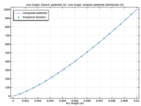
V (SI unit: V) is the potential at the anode, and

•

d (SI unit: m) is the distance between the cathode and the anode.

The comparison between the analytical potential distribution given by Equation 1 and the computed result is shown in Figure 1. The relative error is shown in Figure 2.

The model also includes nodes to compare the total emitted current to the analytical solution given by Equation 2. The relative error in the space charge limited current is about 2%.

Figure 1: Comparison of the computed electric potential and the analytic solution given by Child’s law.

Figure 2: Relative error between the computed electric potential and the analytic solution given by Child’s law.

Reference

1. S. Humphries, Charged Particle Beams, Dover Publications, New York, 2013.

Particle_Tracing_Module/Charged_Particle_Tracing/childs_law_benchmark

Modeling Instructions

From the menu, choose .

New

In the window, click

Model Wizard

In the window, click

In the tree, select .

Click .

Click

In the tree, select .

Click

Global Definitions

Parameters 1

In the window, under click .

In the window for , locate the section.

In the table, enter the following settings:


Name	Expression	Value	Description
V0	1000[V]	1000 V	Potential difference across gap
d	1[cm]	0.01 m	Length of the modeling domain
dbuf	0.01[cm]	1E-4 m	Length of the buffer region
H	2[cm]	0.02 m	Height of the modeling domain
Depth	1[m]	1 m	Depth into the modeling domain
Jan	(4epsilon0_const/9)sqrt(2V0e_const/me_const)*V0/d^2	738.06 A/m²	Analytic current density
Ian	JanHDepth	14.761 A	Analytic total current

Geometry 1

Rectangle 1 (r1)

In the toolbar, click

In the window for , locate the section.

In the text field, type d.

In the text field, type H.

Definitions

Variables 1

In the window, under right-click and choose .

In the window for , locate the section.

In the table, enter the following settings:


Name	Expression	Unit	Description
Van	V0*((x+dbuf)/(d+dbuf))^(4/3)	V	Analytic potential distribution
rel_err	(V-Van)/Van		Error in potential distribution

Materials

Material 1 (mat1)

In the window, under right-click and choose .

In the window for , locate the section.

In the table, enter the following settings:


Property	Variable	Value	Unit	Property group
Relative permittivity	epsilonr_iso ; epsilonrii = epsilonr_iso, epsilonrij = 0	1	1	Basic

Charged Particle Tracing (cpt)

Particle Properties 1

In the window, under click .

In the window for , locate the section.

From the list, choose .

Electric Force 1

In the window, click .

In the window for , locate the section.

From the E list, choose .

Electrostatics (es)

In the window, under click .

Electric Potential 1

In the toolbar, click

and choose .

Select Boundary 4 only.

In the window for , locate the section.

In the V0 text field, type V0.

Multiphysics

Set up space charge limited emission of electrons at the left boundary.

Space Charge Limited Emission 1 (scle1)

In the toolbar, click

and choose .

Select Boundary 1 only.

In the window for , locate the section.

In the os text field, type dbuf.

The iterative scheme employed when solving can be made more stable by ramping up the computed space charge density over a number of iterations. The rate at which the space charge density is ramped up is controlled by the check box in the settings window for the node. Further stability can be achieved by selecting the check box, which treats the charge density as the average over successive iterations. The number of iterations should typically be around 15, depending on the size of the buffer zone specified in the feature. The smaller the buffer zone, the larger the number of iterations should be. In addition, the number of iterations over which to ramp up to full space charge density should be 10-15 less than the number specified in the study settings.

Electric Particle Field Interaction 1 (epfi1)