
|
|
|
|
1
|
|
2
|
In the Select Physics tree, select Acoustics>Acoustic-Structure Interaction>Acoustic-Shell Interaction, Frequency Domain.
|
|
3
|
Click Add.
|
|
4
|
|
5
|
Click Add.
|
|
6
|
|
7
|
Click Add.
|
|
8
|
Click
|
|
9
|
|
10
|
Click
|
|
1
|
|
2
|
|
3
|
|
4
|
|
5
|
Browse to the model’s Application Libraries folder and double-click the file tweeter_shape_optimization_geom_sequence.mph.
|
|
6
|
|
1
|
|
2
|
|
1
|
|
2
|
|
3
|
|
4
|
Browse to the model’s Application Libraries folder and double-click the file tweeter_shape_optimization_model_parameters.txt.
|
|
1
|
|
2
|
|
3
|
|
4
|
Browse to the model’s Application Libraries folder and double-click the file tweeter_shape_optimization_thiele_small_parameters.txt.
|
|
1
|
In the Model Builder window, under Component 1 (comp1) right-click Definitions and choose Variables.
|
|
2
|
|
1
|
|
2
|
|
3
|
|
4
|
|
5
|
|
1
|
|
3
|
|
4
|
|
1
|
In the Model Builder window, expand the Domain Point Probe 1 node, then click Point Probe Expression 1 (ppb1).
|
|
2
|
|
3
|
Locate the Expression section. In the Expression text field, type acpr.Lp_t+10*log10((r_eval/1[m])^2).
|
|
4
|
Select the Description check box.
|
|
5
|
In the associated text field, type Microphone 1 SPL.
|
|
1
|
In the Model Builder window, under Component 1 (comp1)>Definitions right-click Domain Point Probe 1 and choose Duplicate.
|
|
2
|
|
3
|
|
4
|
|
1
|
In the Model Builder window, expand the Domain Point Probe 2 node, then click Point Probe Expression 1 (ppb2).
|
|
2
|
|
3
|
|
1
|
In the Model Builder window, under Component 1 (comp1)>Definitions right-click Domain Point Probe 1 and choose Duplicate.
|
|
2
|
|
3
|
|
4
|
|
1
|
In the Model Builder window, expand the Domain Point Probe 3 node, then click Point Probe Expression 1 (ppb3).
|
|
2
|
|
3
|
|
1
|
In the Model Builder window, under Component 1 (comp1)>Definitions right-click Domain Point Probe 1 and choose Duplicate.
|
|
2
|
|
3
|
|
4
|
|
1
|
In the Model Builder window, expand the Domain Point Probe 4 node, then click Point Probe Expression 1 (ppb4).
|
|
2
|
|
3
|
|
1
|
|
2
|
|
3
|
|
1
|
|
2
|
|
3
|
|
4
|
|
5
|
|
1
|
|
2
|
|
3
|
|
4
|
|
5
|
|
1
|
|
2
|
|
3
|
|
1
|
|
2
|
|
3
|
|
4
|
|
5
|
|
6
|
|
1
|
|
2
|
From the Application Libraries root, browse to the folder Acoustics_Module/Electroacoustic_Transducers and double-click the file loudspeaker_driver_materials.mph.
|
|
3
|
Click
|
|
1
|
|
2
|
In the tree, select Built-in>Air.
|
|
3
|
|
4
|
|
5
|
|
6
|
|
7
|
|
8
|
|
9
|
|
10
|
|
11
|
|
12
|
|
1
|
|
2
|
|
3
|
|
1
|
|
2
|
|
3
|
|
1
|
|
2
|
|
3
|
|
4
|
|
1
|
|
2
|
|
3
|
|
4
|
|
1
|
|
2
|
|
3
|
|
1
|
In the Model Builder window, under Component 1 (comp1) click Pressure Acoustics, Frequency Domain (acpr).
|
|
2
|
In the Settings window for Pressure Acoustics, Frequency Domain, locate the Domain Selection section.
|
|
3
|
|
1
|
|
2
|
|
3
|
|
4
|
|
5
|
|
1
|
|
2
|
|
3
|
|
4
|
Locate the Porous Matrix Properties section. From the Rf list, choose User defined. In the associated text field, type rf_pa.
|
|
5
|
|
1
|
|
2
|
|
3
|
|
4
|
Locate the Exterior Field Calculation section. From the Condition in the z = z^0 plane list, choose Symmetric/Infinite sound hard boundary.
|
|
1
|
|
2
|
|
3
|
|
1
|
|
2
|
|
3
|
|
1
|
|
2
|
|
3
|
|
4
|
|
5
|
|
6
|
|
7
|
|
8
|
|
1
|
|
2
|
|
3
|
|
1
|
|
2
|
|
3
|
|
4
|
|
1
|
|
2
|
|
3
|
|
4
|
|
1
|
|
2
|
|
3
|
|
1
|
|
2
|
|
3
|
|
1
|
|
2
|
|
3
|
|
4
|
|
5
|
|
1
|
|
2
|
|
4
|
|
1
|
|
2
|
|
4
|
|
1
|
|
2
|
|
4
|
|
1
|
|
2
|
|
4
|
|
1
|
|
2
|
|
4
|
|
1
|
|
2
|
|
4
|
|
1
|
In the Model Builder window, under Component 1 (comp1) right-click Multiphysics and choose Acoustic-Structure Boundary.
|
|
2
|
|
3
|
|
4
|
|
1
|
|
2
|
|
3
|
|
1
|
|
2
|
|
3
|
|
1
|
|
2
|
|
3
|
|
4
|
|
5
|
|
6
|
In the associated text field, type air_gap.
|
|
1
|
|
2
|
|
3
|
Click the Custom button.
|
|
4
|
|
5
|
|
6
|
|
1
|
|
2
|
|
3
|
|
1
|
|
2
|
|
3
|
|
4
|
|
5
|
|
6
|
|
7
|
In the associated text field, type mesh_optim.
|
|
1
|
|
2
|
|
3
|
|
1
|
|
2
|
|
3
|
|
4
|
|
1
|
|
3
|
|
4
|
|
5
|
|
1
|
|
2
|
|
3
|
|
5
|
|
1
|
|
2
|
|
3
|
|
4
|
|
5
|
|
1
|
|
2
|
|
3
|
|
1
|
|
2
|
|
3
|
|
4
|
|
5
|
Locate the Physics and Variables Selection section. In the table, clear the Solve for check box for Deformed geometry (Component 1).
|
|
6
|
|
1
|
|
2
|
|
3
|
|
4
|
|
1
|
|
2
|
|
3
|
In the Settings window for Solution, type Study 1 - Initial Design/Revolution in the Label text field.
|
|
1
|
|
2
|
|
3
|
|
4
|
|
1
|
|
2
|
In the Settings window for Revolution 2D, type Revolution 2D - Initial Design in the Label text field.
|
|
3
|
|
4
|
|
5
|
|
6
|
|
1
|
|
2
|
|
3
|
|
1
|
|
2
|
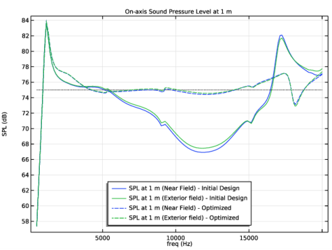
In the Settings window for 1D Plot Group, type On-axis Sound Pressure Level at 1 m in the Label text field.
|
|
3
|
|
4
|
|
5
|
In the associated text field, type freq (Hz).
|
|
6
|
|
7
|
In the associated text field, type SPL (dB).
|
|
8
|
|
1
|
|
2
|
|
4
|
|
1
|
|
2
|
|
3
|
|
4
|
|
5
|
Select the Description check box.
|
|
6
|
In the associated text field, type SPL at 1 m (Exterior field) - Initial Design.
|
|
7
|
|
8
|
|
9
|
|
1
|
|
2
|
|
4
|
Click to expand the Coloring and Style section. Find the Line style subsection. From the Line list, choose Dotted.
|
|
5
|
|
6
|
|
7
|
|
1
|
|
2
|
|
3
|
|
1
|
|
2
|
|
3
|
|
4
|
|
5
|
Locate the Evaluation section. Find the Angles subsection. From the Restriction list, choose Manual.
|
|
6
|
|
7
|
|
8
|
|
9
|
|
10
|
|
11
|
|
12
|
|
13
|
|
1
|
|
2
|
|
3
|
|
4
|
|
5
|
|
6
|
|
7
|
|
8
|
|
1
|
|
2
|
|
3
|
|
4
|
|
5
|
|
1
|
|
2
|
|
3
|
|
1
|
|
2
|
|
3
|
|
4
|
|
1
|
|
2
|
|
3
|
|
4
|
|
5
|
|
1
|
|
2
|
|
3
|
|
4
|
|
1
|
In the Model Builder window, under Results>Sound Pressure Level right-click Line 1 and choose Duplicate.
|
|
2
|
|
3
|
|
4
|
|
1
|
|
2
|
|
3
|
|
4
|
|
5
|
|
1
|
|
2
|
|
3
|
|
1
|
|
2
|
|
3
|
|
4
|
|
5
|
|
1
|
|
2
|
|
3
|
|
4
|
|
1
|
|
2
|
|
3
|
|
4
|
|
1
|
|
2
|
|
3
|
|
1
|
|
2
|
|
3
|
|
4
|
|
6
|
|
1
|
|
2
|
|
3
|
In the Frequencies text field, type range(fmin_optim,(fmax_optim-fmin_optim)/(nf_optim-1),fmax_optim).
|
|
4
|
|
1
|
|
2
|
|
3
|
|
4
|
|
1
|
|
2
|
|
3
|
|
4
|
|
5
|
|
6
|
|
7
|
|
8
|
|
1
|
|
2
|
|
3
|
|
4
|
|
5
|
|
1
|
|
2
|
|
3
|
|
4
|
|
5
|
|
6
|
|
7
|
|
1
|
|
2
|
|
3
|
|
4
|
|
5
|
|
6
|
|
1
|
|
2
|
|
3
|
Select the Plot check box.
|
|
4
|
|
5
|
|
1
|
|
2
|
|
3
|
|
4
|
|
1
|
|
2
|
|
3
|
Locate the Physics and Variables Selection section. In the table, clear the Solve for check box for Deformed geometry (Component 1).
|
|
4
|
Click to expand the Values of Dependent Variables section. Find the Initial values of variables solved for subsection. From the Settings list, choose User controlled.
|
|
5
|
|
6
|
|
7
|
Find the Values of variables not solved for subsection. From the Settings list, choose User controlled.
|
|
8
|
|
9
|
|
10
|
|
11
|
|
12
|
|
13
|
|
14
|
|
15
|
|
1
|
|
2
|
|
3
|
|
4
|
|
1
|
|
2
|
In the Settings window for Solution, type Study 3 - Optimized Design/Revolution in the Label text field.
|
|
1
|
In the Model Builder window, expand the Results>Datasets>Study 3 - Optimized Design/Revolution (sol3) node, then click Selection.
|
|
2
|
|
3
|
|
4
|
|
1
|
|
2
|
In the Settings window for Revolution 2D, type Revolution 2D - Optimized Design in the Label text field.
|
|
3
|
Locate the Data section. From the Dataset list, choose Study 3 - Optimized Design/Revolution (sol3).
|
|
4
|
|
5
|
|
1
|
In the Model Builder window, under Results>On-axis Sound Pressure Level at 1 m right-click Global 1 and choose Duplicate.
|
|
2
|
|
3
|
|
4
|
|
5
|
Locate the Coloring and Style section. Find the Line style subsection. From the Line list, choose Dashed.
|
|
6
|
|
1
|
In the Model Builder window, under Results>On-axis Sound Pressure Level at 1 m right-click Octave Band 1 and choose Duplicate.
|
|
2
|
|
3
|
|
4
|
Locate the y-Axis Data section. In the Description text field, type SPL at 1 m (Exterior field) - Optimized.
|
|
5
|
Click to expand the Coloring and Style section. Find the Line style subsection. From the Line list, choose Dashed.
|
|
1
|
In the Model Builder window, under Results>Directivity right-click Directivity 1 and choose Duplicate.
|
|
2
|
|
3
|
|
4
|
|
5
|
|
1
|
In the Model Builder window, under Results>Directivity right-click Directivity 2 and choose Duplicate.
|
|
2
|
|
3
|
|
4
|
|
5
|
|
1
|
|
2
|
|
4
|
Locate the y-Coordinates section. In the table, enter the following settings:
|
|
5
|
Click to expand the Coloring and Style section. Find the Line style subsection. From the Line list, choose Dashed.
|
|
6
|
|
7
|
|
8
|
|
1
|
|
2
|
|
4
|
Locate the y-Coordinates section. In the table, enter the following settings:
|
|
5
|
Locate the Coloring and Style section. Find the Line style subsection. From the Line list, choose Dash-dot.
|
|
6
|
|
7
|
|
8
|
|
1
|
|
2
|
|
3
|
|
4
|
|
5
|
|
6
|
|
7
|
|
1
|
|
2
|
|
3
|
|
4
|
|
5
|
|
6
|
|
1
|
|
2
|
|
3
|
|
4
|
|
5
|
|
6
|
|
1
|
|
2
|
|
3
|
|
4
|
|
5
|
|
6
|
|
7
|
|
8
|
Click Define custom colors.
|
|
10
|
Click Add to custom colors.
|
|
11
|
|
1
|
|
2
|
|
3
|
|
4
|
|
1
|
|
2
|
|
3
|
|
4
|
|
5
|
|
6
|
|
7
|
|
8
|
|
1
|
|
2
|
|
3
|
|
4
|
|
5
|
|
6
|
|
7
|
|
1
|
|
2
|
Click
|
|
1
|
|
2
|
|
3
|
|
4
|
Browse to the model’s Application Libraries folder and double-click the file tweeter_shape_optimization_geometry_parameters.txt.
|
|
1
|
|
2
|
|
3
|
|
1
|
|
2
|
|
3
|
|
4
|
|
5
|
Click to expand the Layers section. Locate the Position section. In the z text field, type -h_former+h_voice_coil/2-h_top_plate/2-h_back-h_waveguide.
|
|
6
|
Locate the Layers section. In the table, enter the following settings:
|
|
7
|
|
8
|
|
9
|
|
10
|
|
1
|
|
2
|
|
3
|
|
4
|
|
5
|
|
6
|
|
7
|
Locate the Layers section. In the table, enter the following settings:
|
|
8
|
|
9
|
|
10
|
|
11
|
|
1
|
|
2
|
|
3
|
|
4
|
Locate the Coordinates section. In the table, enter the following settings:
|
|
5
|
|
1
|
|
2
|
|
4
|
Locate the End Conditions section. From the Condition at starting point list, choose Tangent direction.
|
|
5
|
|
6
|
|
7
|
|
8
|
|
9
|
|
10
|
|
1
|
|
2
|
|
4
|
Locate the End Conditions section. From the Condition at starting point list, choose Tangent direction.
|
|
5
|
|
6
|
|
7
|
|
8
|
|
9
|
|
10
|
|
1
|
|
2
|
|
3
|
On the object ic1, select Point 2 only.
|
|
4
|
Locate the Endpoint section. Find the End vertex subsection. Select the
|
|
5
|
On the object r2, select Point 3 only.
|
|
6
|
Locate the Selections of Resulting Entities section. Select the Resulting objects selection check box.
|
|
7
|
|
1
|
|
2
|
On the object ic2, select Point 2 only.
|
|
3
|
|
4
|
|
5
|
|
6
|
|
1
|
|
2
|
|
3
|
|
4
|
|
5
|
|
6
|
|
7
|
|
1
|
|
2
|
|
3
|
|
4
|
|
5
|
|
6
|
|
7
|
|
8
|
|
1
|
|
2
|
|
3
|
|
4
|
|
5
|
|
6
|
|
7
|
|
1
|
|
2
|
|
3
|
|
4
|
|
5
|
Locate the Point on Line of Reflection section. In the z text field, type (-h_former+h_voice_coil/2+h_top_plate/2)/2 -h_waveguide.
|
|
6
|
|
7
|
|
8
|
|
1
|
|
2
|
|
3
|
|
4
|
Locate the Coordinates section. In the table, enter the following settings:
|
|
5
|
|
1
|
|
2
|
|
3
|
|
4
|
|
5
|
Locate the Position section. In the z text field, type -h_former+h_voice_coil/2+h_top_plate/2-h_waveguide.
|
|
6
|
Locate the Selections of Resulting Entities section. Select the Resulting objects selection check box.
|
|
7
|
|
1
|
|
2
|
Select the object r1 only.
|
|
3
|
|
4
|
|
1
|
|
2
|
|
3
|
|
4
|
On the object uni1, select Domains 1, 13, and 14 only.
|
|
5
|
|
1
|
|
2
|
|
3
|
On the object del1, select Domains 5, 12, and 13 only.
|
|
1
|
|
2
|
|
3
|
On the object del1, select Domain 8 only.
|
|
1
|
|
2
|
|
3
|
|
4
|
|
5
|
Click OK.
|
|
1
|
|
2
|
|
3
|
On the object del1, select Domains 7 and 11 only.
|
|
1
|
|
2
|
|
3
|
On the object del1, select Domains 1–3, 6, 7, and 9–11 only.
|
|
1
|
|
2
|
|
3
|
|
4
|
On the object del1, select Boundaries 9 and 39 only.
|
|
1
|
|
2
|
|
3
|
|
4
|
On the object del1, select Boundary 46 only.
|
|
1
|
|
2
|
In the Settings window for Explicit Selection, type Symmetry/Roller Boundaries in the Label text field.
|
|
3
|
|
4
|
On the object del1, select Boundaries 3 and 5 only.
|
|
1
|
|
2
|
|
3
|
|
4
|
On the object del1, select Boundaries 47–52 only.
|
|
1
|
|
2
|
|
3
|
|
4
|
On the object del1, select Boundaries 2, 4, 11–15, 17, 19–25, 28–36, and 46–53 only.
|
|
1
|
|
2
|
|
3
|
|
4
|
|
5
|
|
6
|
Click OK.
|
|
1
|
|
2
|
|
3
|
|
4
|
On the object del1, select Boundary 53 only.
|
|
1
|
|
2
|
|
3
|
|
4
|
On the object del1, select Points 31 and 32 only.
|
|
1
|
|
2
|
Find the Studies subsection. In the Select Study tree, select Preset Studies for Selected Physics Interfaces>Stationary.
|
|
3
|
|
4
|
|
1
|
|
2
|
|
3
|
|
4
|
|
5
|
|
1
|
|
2
|
|
3
|
|
1
|
|
2
|
|
3
|
|
4
|
|
1
|
In the Model Builder window, under Results>Datasets right-click Revolution 2D 1 and choose Duplicate.
|
|
2
|
|
3
|
|
1
|
|
2
|
|
3
|
|
1
|
|
2
|
|
3
|
|
4
|
|
5
|
|
6
|
|
1
|
|
2
|
|
3
|
|
4
|
|
5
|
|
1
|
|
2
|
|
3
|
|
4
|
|
5
|
|
6
|
|
7
|
|
8
|
Locate the Expression section. In the Expression text field, type if((rev1phi>-90[deg])*(rev1phi<135[deg]),1,0).
|
|
9
|
|
10
|
|
11
|
|
12
|
|
13
|
|
14
|
|
15
|
|
16
|
|
17
|
|
1
|
|
2
|
|
3
|
|
4
|
|
5
|
|
6
|
|
1
|
|
2
|
|
3
|
|
1
|
|
2
|
|
3
|
|
4
|
|
1
|
|
2
|
|
3
|
In the Logical expression for inclusion text field, type (rev1phi>-90[deg])*(rev1phi<135[deg])*(r>0).
|
|
4
|
|
1
|
In the Model Builder window, under Results>Datasets right-click Revolution 2D 2 and choose Duplicate.
|
|
2
|
|
3
|
|
1
|
|
2
|
|
3
|
|
4
|
|
5
|
|
6
|
|
7
|
|
1
|
|
2
|
|
3
|
|
1
|
In the Model Builder window, under Results>Datasets right-click Revolution 2D 3 and choose Duplicate.
|
|
2
|
|
3
|
|
1
|
|
2
|
|
3
|
|
4
|
|
5
|
|
6
|
|
7
|
Click Define custom colors.
|
|
9
|
Click Add to custom colors.
|
|
10
|
|
1
|
|
2
|
|
3
|
|
1
|
In the Model Builder window, under Results>Datasets right-click Revolution 2D 4 and choose Duplicate.
|
|
2
|
|
3
|
|
1
|
In the Model Builder window, under Results>3D Plot Group 1 right-click Surface 1 and choose Duplicate.
|
|
2
|
|
3
|
|
4
|
Locate the Coloring and Style section. On Windows, click the colored bar underneath, or — if you are running the cross-platform desktop — the Color button.
|
|
5
|
Click Define custom colors.
|
|
7
|
Click Add to custom colors.
|
|
8
|
|
1
|
|
1
|
|
2
|
|
3
|
|
1
|
In the Model Builder window, under Results>Datasets right-click Revolution 2D 5 and choose Duplicate.
|
|
2
|
|
3
|
|
1
|
In the Model Builder window, under Results>3D Plot Group 1 right-click Surface 2 and choose Duplicate.
|
|
2
|
|
3
|
|
4
|
Locate the Coloring and Style section. On Windows, click the colored bar underneath, or — if you are running the cross-platform desktop — the Color button.
|
|
5
|
Click Define custom colors.
|
|
7
|
Click Add to custom colors.
|
|
8
|
|
1
|
|
2
|
|
3
|
|
4
|
|
5
|
|
6
|
|
7
|
|
8
|
Click Define custom colors.
|
|
10
|
Click Add to custom colors.
|
|
11
|
|
12
|
|
1
|
|
2
|
|
3
|
|
1
|
In the Model Builder window, under Results>Datasets right-click Revolution 2D 6 and choose Duplicate.
|
|
2
|
|
3
|
|
1
|
In the Model Builder window, under Results>3D Plot Group 1 right-click Surface 4 and choose Duplicate.
|
|
2
|
|
3
|
|
4
|
Locate the Coloring and Style section. On Windows, click the colored bar underneath, or — if you are running the cross-platform desktop — the Color button.
|
|
5
|
Click Define custom colors.
|
|
7
|
Click Add to custom colors.
|
|
8
|
|
9
|
|
1
|
|
2
|
|
3
|
|
1
|
In the Model Builder window, under Results>Datasets right-click Revolution 2D 7 and choose Duplicate.
|
|
2
|
|
3
|
|
1
|
In the Model Builder window, under Results>3D Plot Group 1 right-click Surface 5 and choose Duplicate.
|
|
2
|
|
3
|
|
4
|
Locate the Coloring and Style section. On Windows, click the colored bar underneath, or — if you are running the cross-platform desktop — the Color button.
|
|
5
|
Click Define custom colors.
|
|
7
|
Click Add to custom colors.
|
|
8
|
|
1
|
|
2
|
|
3
|
|
1
|
|
2
|
|
3
|
|
1
|
|
2
|
|
3
|
|
1
|
In the Model Builder window, under Results>Datasets right-click Revolution 2D 7 and choose Duplicate.
|
|
2
|
|
3
|
|
1
|
In the Model Builder window, under Results>3D Plot Group 1 right-click Surface 1 and choose Duplicate.
|
|
2
|
|
3
|
|
4
|
Locate the Coloring and Style section. On Windows, click the colored bar underneath, or — if you are running the cross-platform desktop — the Color button.
|
|
5
|
Click Define custom colors.
|
|
7
|
Click Add to custom colors.
|
|
8
|
|
1
|
|
2
|
|
3
|
|
4
|
|
5
|
|
6
|