|
|
|
|
•
|
|
•
|
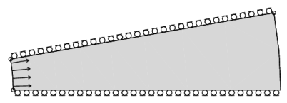
An internal pressure of 30 MPa.
|
|
•
|

|
1
|
|
2
|
|
3
|
Click Add.
|
|
4
|
Click
|
|
5
|
|
6
|
Click
|
|
1
|
|
2
|
|
1
|
|
2
|
|
3
|
|
4
|
|
5
|
|
6
|
|
1
|
|
2
|
|
3
|
|
4
|
|
5
|
|
1
|
|
2
|
Select the object c1 only.
|
|
3
|
|
4
|
|
5
|
Select the object c2 only.
|
|
6
|
|
7
|
|
1
|
|
2
|
|
3
|
|
4
|
|
5
|
|
1
|
|
1
|
|
3
|
|
4
|
|
5
|
|
6
|
|
7
|
|
8
|
From the list, choose Quasistatic.
|
|
1
|
In the Model Builder window, under Component 1 (comp1) right-click Materials and choose Blank Material.
|
|
2
|
|
1
|
|
2
|
|
3
|
|
4
|
|
1
|
|
2
|
|
3
|
|
4
|
|
5
|
Click
|
|
6
|
|
7
|
|
8
|
|
9
|
|
10
|
Click Add.
|
|
11
|
|
12
|
|
13
|
|
1
|
|
2
|
|
3
|
|
4
|
|
5
|
|
6
|
|
7
|
Click
|
|
1
|
|
2
|
|
1
|
|
2
|
|
3
|
|
4
|
|
5
|
|
1
|
|
2
|
|
3
|
|
1
|
|
2
|
|
3
|
|
1
|
|
3
|
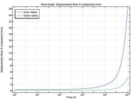
In the Settings window for Point Graph, click Replace Expression in the upper-right corner of the y-Axis Data section. From the menu, choose Component 1 (comp1)>Solid Mechanics>Displacement>Displacement field - m>u - Displacement field, R component.
|
|
4
|
|
5
|
|
6
|
|
1
|
|
2
|
|
3
|
|
4
|
|
1
|
|
2
|
|
3
|
|
4
|
|
1
|
|
2
|
|
3
|
|
4
|
|
1
|
|
2
|
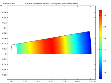
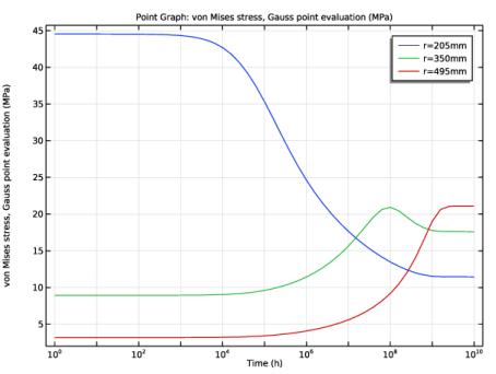
In the Settings window for Point Graph, click Replace Expression in the upper-right corner of the y-Axis Data section. From the menu, choose Component 1 (comp1)>Solid Mechanics>Stress (Gauss points)>solid.misesGp - von Mises stress, Gauss point evaluation - N/m².
|
|
3
|
|
4
|
|
5
|
|
7
|