PDF

Combining Creep Material Models
Introduction
This model illustrates how to combine different creep models to accurately represent the material behavior. An example for such a material model combination is to add a Norton-Bailey’s law with a Norton’s law as described in the equation
Model Definition
This model is a modification of the application library model Thermally Induced Creep. The same geometry, hollow sphere, load, inner pressure and thermal gradient, are used here. The parameters of Norton’s law are also reused and govern secondary creep. The primary creep data, which differentiates the two models, is defined as
Parameter A2 = 10 h-1 accounts for the stress normalization of the equivalent stress, σe, in MPa and time, t, in hours. The other parameters are n2 = 3.5, m = 0.5, and
f2(T) = e-12500/T, where T defines the temperature in K .
Results and Discussion
Figure 1 shows the von Mises stress at 108 h when both primary creep and secondary creep are active. The largest equivalent stress, found in the center of the sphere, demonstrates that the relaxation take place starting from the inner radius and continuing toward the outer boundary. Without creep due to the internal pressure, the largest stresses are found on the inner radius and decreases toward the outer radius instead.
Figure 1: Distribution of von Mises stress at t = 108 h.
To compare the both creep models, secondary creep against combined creep, see Figure 2 where the time history of the equivalent stress is shown at three different locations. It is clear that the primary creep relaxes the inner boundary earlier than the secondary creep; compare the turquoise and blue lines. Over time, both creep models converge to the same result. This is expected because the influence of the primary creep fades away with time.
The creep strain can also be plotted for primary and secondary creep separately. The primary creep strain increases earlier than secondary creep, as shown in Figure 3. Lastly, the history of the stress profile is shown in Figure 4. Relaxation causes the propagation from the inner to the outer radius of the position of the peak stress.
Figure 2: History of von Mises stress at radius 205 mm, 350 mm, and 495 mm, of the secondary creep only (solid lines), and with primary creep included (dashed lines).
Figure 3: History of primary and secondary creep strain at radius 205 mm, 350 mm, and 495 mm.
Figure 4: von Mises stress versus radius at t = 1, 104, 105, 107, 108, and 1010 hours with primary creep included.
Modeling in COMSOL Multiphysics
In COMSOL Multiphysics you can add several Creep nodes under the same Linear Elastic Material feature. Each creep node can define its unique creep model.
The Norton-Bailey’s law is defied in Nonlinear Structural Materials Module with
In order to normalize the equivalent stress in MPa and the time in h, set the reference stress σref = 1 MPa and the reference time tref = 1 h. Set the time shift tshift to 1 min in order to avoid the singularity that occurs at t = 0. Considering the long time scale of the analysis this has a negligible effect on the results.
Application Library path: Nonlinear_Structural_Materials_Module/Creep/combined_creep
Modeling Instructions
From the File menu, choose Open.
Browse to the model’s Application Libraries folder and double-click the file thermally_induced_creep.mph.
Component 1 (comp1)
In the Model Builder window, expand the Component 1 (comp1) node.
Solid Mechanics (solid)
Linear Elastic Material 1
In the Model Builder window, expand the Component 1 (comp1)>Solid Mechanics (solid) node, then click Linear Elastic Material 1.
Creep 2
1
In the Physics toolbar, click  Attributes and choose Creep.
2
In the Settings window for Creep, locate the Creep Data section.
3
From the Material model list, choose Norton-Bailey.
4
From the A list, choose User defined. In the associated text field, type 10[1/h].
5
From the σref list, choose User defined. From the n list, choose User defined. In the associated text field, type 3.5.
6
In the m text field, type 0.5.
7
In the tshift text field, type 1[min].
8
Select the Include temperature dependency check box.
9
In the Q text field, type 1.0393e5[J/mol].
10
Locate the Model Input section. From the T list, choose User defined. In the associated text field, type T.
Study 1 solves the model with only Creep 1 enabled. Disable Creep 2 for this study.
Study 1
Step 1: Time Dependent
1
In the Model Builder window, expand the Study 1 node, then click Step 1: Time Dependent.
2
In the Settings window for Time Dependent, locate the Physics and Variables Selection section.
3
Select the Modify model configuration for study step check box.
4
In the Physics and variables selection tree, select Component 1 (comp1)>Solid Mechanics (solid)>Linear Elastic Material 1>Creep 2.
5
Click  Disable.
Add a new study to solve for the combined creep.
Add Study
1
In the Home toolbar, click  Add Study to open the Add Study window.
2
Go to the Add Study window.
3
Find the Studies subsection. In the Select Study tree, select General Studies>Time Dependent.
4
Click Add Study in the window toolbar.
5
In the Home toolbar, click  Add Study to close the Add Study window.
Study 2
Step 1: Time Dependent
1
In the Settings window for Time Dependent, locate the Study Settings section.
2
From the Time unit list, choose h.
3
In the Output times text field, type 0 10^{range(0,0.2,10)}.
4
From the Tolerance list, choose User controlled.
5
In the Relative tolerance text field, type 1e-4.
Solution 2 (sol2)
1
In the Study toolbar, click  Show Default Solver.
2
In the Model Builder window, expand the Solution 2 (sol2) node, then click Time-Dependent Solver 1.
3
In the Settings window for Time-Dependent Solver, click to expand the Time Stepping section.
4
Select the Initial step check box.
5
6
From the Steps taken by solver list, choose Strict.
7
In the Study toolbar, click  Compute.
Results
Stress with Combined Creep
Select the solution at 108 hours to reproduce Figure 1.
1
In the Settings window for 2D Plot Group, type Stress with Combined Creep in the Label text field.
2
Locate the Data section. From the Time (h) list, choose 1E8.
Surface 1
1
In the Model Builder window, expand the Stress with Combined Creep node, then click Surface 1.
2
In the Settings window for Surface, locate the Expression section.
3
From the Unit list, choose MPa.
4
In the Stress with Combined Creep toolbar, click  Plot.
5
Click the  Zoom Extents button in the Graphics toolbar.
The commands below illustrate how to generate Figure 2.
Stress with Combined Creep, 3D
1
In the Model Builder window, under Results click Stress, 3D (solid) 1.
2
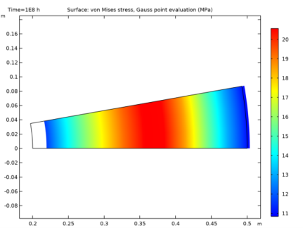
In the Settings window for 3D Plot Group, type Stress with Combined Creep, 3D in the Label text field.
3
Locate the Data section. From the Time (h) list, choose 1E8.
Surface 1
1
In the Model Builder window, expand the Stress with Combined Creep, 3D node, then click Surface 1.
2
In the Settings window for Surface, locate the Expression section.
3
From the Unit list, choose MPa.
4
In the Stress with Combined Creep, 3D toolbar, click  Plot.
Cut Point 2D 2
1
In the Model Builder window, expand the Results>Datasets node.
2
Right-click Results>Datasets>Cut Point 2D 1 and choose Duplicate.
3
In the Settings window for Cut Point 2D, locate the Data section.
4
From the Dataset list, choose Study 2/Solution 2 (sol2).
Point Graph 1
1
In the Model Builder window, expand the Results>von Mises Stress node, then click Point Graph 1.
2
In the Settings window for Point Graph, click to expand the Legends section.
3
Point Graph 2
1
Right-click Results>von Mises Stress>Point Graph 1 and choose Duplicate.
2
In the Settings window for Point Graph, locate the Data section.
3
From the Dataset list, choose Cut Point 2D 2.
4
Click to expand the Title section. From the Title type list, choose None.
5
Click to expand the Coloring and Style section. Find the Line style subsection. From the Line list, choose Dashed.
6
From the Color list, choose Cycle (reset).
7
Locate the Legends section. In the table, enter the following settings:
8
In the von†Mises Stress toolbar, click  Plot.
To get Figure 4, continue with the steps below:
Cut Line 2D 1
1
In the Results toolbar, click  Cut Line 2D.
2
In the Settings window for Cut Line 2D, locate the Data section.
3
From the Dataset list, choose Study 2/Solution 2 (sol2).
4
Locate the Line Data section. In row Point 1, set R to 0.2.
5
In row Point 2, set R to 0.5.
von Mises Stress, Profile
1
In the Results toolbar, click  1D Plot Group.
2
In the Settings window for 1D Plot Group, type von†Mises Stress, Profile in the Label text field.
3
Locate the Data section. From the Dataset list, choose Cut Line 2D 1.
4
From the Time selection list, choose From list.
5
In the Times (h) list, choose 1, 10000, 1E5, 1E7, 1E8, and 1E10.
Line Graph 1
1
Right-click von Mises Stress, Profile and choose Line Graph.
2
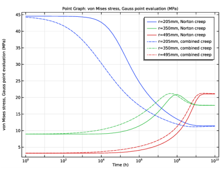
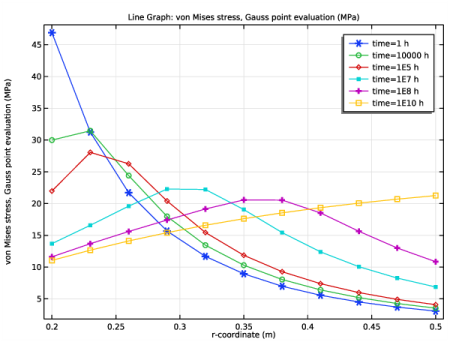
In the Settings window for Line Graph, click Replace Expression in the upper-right corner of the y-Axis Data section. From the menu, choose Component 1 (comp1)>Solid Mechanics>Stress (Gauss points)>solid.misesGp - von Mises stress, Gauss point evaluation - N/m².
3
Locate the y-Axis Data section. From the Unit list, choose MPa.
4
Locate the x-Axis Data section. From the Parameter list, choose Expression.
5
In the Expression text field, type r.
6
Click to expand the Coloring and Style section. Find the Line markers subsection. From the Marker list, choose Cycle.
7
From the Positioning list, choose In data points.
8
Click to expand the Quality section. From the Resolution list, choose No refinement.
9
Click to expand the Legends section. Select the Show legends check box.
10
Find the Include subsection. In the Prefix text field, type time=.
11
In the von†Mises Stress, Profile toolbar, click  Plot.
Primary and secondary creep strain can be plotted separately, see Figure 3.
Creep Strains
1
In the Home toolbar, click  Add Plot Group and choose 1D Plot Group.
2
In the Settings window for 1D Plot Group, type Creep Strains in the Label text field.
Point Graph 1
1
In the Creep Strains toolbar, click  Point Graph.
2
In the Settings window for Point Graph, locate the Data section.
3
From the Dataset list, choose Cut Point 2D 2.
4
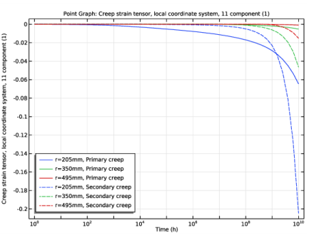
Click Replace Expression in the upper-right corner of the y-Axis Data section. From the menu, choose Component 1 (comp1)>Solid Mechanics>Strain (Gauss points)>Creep strain tensor, local coordinate system>solid.lemm1.cmm2.ecGp11 - Creep strain tensor, local coordinate system, 11 component.
5
Locate the Legends section. Select the Show legends check box.
6
From the Legends list, choose Manual.
7
Point Graph 2
1
Right-click Point Graph 1 and choose Duplicate.
2
In the Settings window for Point Graph, click Replace Expression in the upper-right corner of the y-Axis Data section. From the menu, choose Component 1 (comp1)>Solid Mechanics>Strain (Gauss points)>Creep strain tensor, local coordinate system>solid.lemm1.cmm1.ecGp11 - Creep strain tensor, local coordinate system, 11 component.
3
Locate the Coloring and Style section. Find the Line style subsection. From the Line list, choose Dashed.
4
From the Color list, choose Cycle (reset).
5
Locate the Legends section. In the table, enter the following settings:
6
Locate the Title section. From the Title type list, choose None.
7
Click the  x-Axis Log Scale button in the Graphics toolbar.
Creep Strains
1
In the Model Builder window, click Creep Strains.
2
In the Settings window for 1D Plot Group, locate the Legend section.
3
From the Position list, choose Lower left.
4
In the Creep Strains toolbar, click  Plot.