|
|
|
|
1
|
|
2
|
|
3
|
|
4
|
|
5
|
|
1
|
In the Model Builder window, under Component 1 (comp1) right-click Materials and choose Blank Material.
|
|
2
|
|
4
|
|
1
|
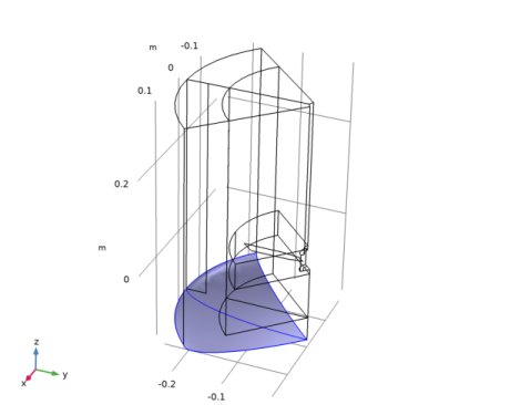
In the Model Builder window, under Component 1 (comp1)>Definitions>Moving Mesh click Rotating Domain 1.
|
|
2
|
|
3
|
|
4
|
|
1
|
In the Model Builder window, under Component 1 (comp1) right-click Laminar Flow (spf) and choose Interior Wall.
|
|
2
|
|
3
|
|
1
|
|
2
|
|
3
|
|
1
|
|
2
|
|
3
|
|
1
|
|
2
|
|
3
|
|
1
|
|
2
|
|
1
|
|
2
|
|
3
|
|
4
|
|
1
|
|
2
|
|
3
|
|
4
|
|
1
|
|
2
|
|
1
|
|
2
|
|
3
|
Find the Studies subsection. In the Select Study tree, select Preset Studies for Selected Physics Interfaces>Frozen Rotor.
|
|
4
|
|
5
|
|
1
|
|
2
|
|
3
|
|
1
|
|
2
|
|
3
|
|
4
|
|
5
|
|
6
|
|
7
|
|
8
|
|
9
|
Click
|
|
1
|
|
2
|
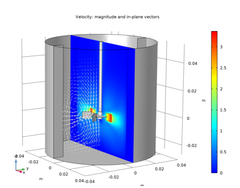
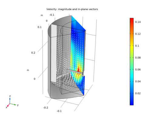
In the Settings window for 3D Plot Group, type Velocity: Magnitude and Vectors in the Label text field.
|
|
3
|
|
1
|
|
2
|
Click Yes to confirm.
|
|
1
|
|
2
|
Click Yes to confirm.
|
|
1
|
|
2
|
Click Yes to confirm.
|
|
1
|
|
2
|
|
3
|
|
4
|
|
1
|
|
2
|
|
3
|
|
4
|
|
5
|
|
6
|
|
7
|
|
8
|
|
9
|
|
1
|
|
2
|
|
3
|
|
4
|
|
5
|
|
1
|
|
2
|
|
3
|
|
4
|
Click OK.
|
|
5
|
|
7
|
Click
|
|
1
|
|
2
|
|
3
|
|
4
|
Click OK.
|
|
5
|
|
7
|
Click
|
|
1
|
|
2
|
|
3
|
|
4
|
Click OK.
|
|
5
|
|
6
|
|
7
|
Locate the Expressions section. In the table, enter the following settings:
|
|
8
|
Click
|
|
1
|
|
2
|
Browse to the model’s Application Libraries folder and double-click the file modular_mixer_turbulent_geom.mph.
|
|
1
|
|
2
|
|
3
|
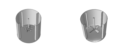
In the tree, select Fluid Flow>Single-Phase Flow>Rotating Machinery, Fluid Flow>Turbulent Flow>Turbulent Flow, k-ε.
|
|
4
|
|
5
|
|
1
|
|
2
|
|
3
|
|
4
|
|
5
|
|
1
|
In the Model Builder window, under Component 1 (comp1) right-click Turbulent Flow, k-ε (spf) and choose Interior Wall.
|
|
2
|
|
3
|
|
1
|
|
2
|
|
3
|
|
1
|
|
2
|
|
3
|
|
1
|
|
1
|
|
2
|
|
3
|
|
1
|
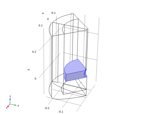
In the Model Builder window, under Component 1 (comp1)>Definitions>Moving Mesh click Rotating Domain 1.
|
|
2
|
|
3
|
|
4
|
|
1
|
|
2
|
|
1
|
|
2
|
|
3
|
|
4
|
|
1
|
|
2
|
|
3
|
|
4
|
|
1
|
In the Model Builder window, under Component 1 (comp1) right-click Mesh 1 and choose Edit Physics-Induced Sequence.
|
|
2
|
|
3
|
Click the Custom button.
|
|
4
|
|
1
|
|
2
|
|
4
|
|
1
|
|
2
|
|
3
|
|
5
|
|
6
|
|
7
|
Click the Custom button.
|
|
8
|
|
1
|
|
2
|
|
3
|
|
5
|
|
6
|
|
7
|
Click the Custom button.
|
|
8
|
|
9
|
|
10
|
|
11
|
In the associated text field, type 0.00123.
|
|
12
|
|
13
|
|
1
|
|
2
|
|
3
|
|
5
|
|
6
|
|
7
|
|
8
|
|
9
|
|
1
|
|
2
|
|
3
|
Find the Studies subsection. In the Select Study tree, select Preset Studies for Selected Physics Interfaces>Frozen Rotor.
|
|
4
|
|
5
|
|
1
|
|
2
|
|
3
|
|
4
|
|
5
|
|
6
|
|
7
|
Click
|
|
1
|
|
2
|
|
1
|
|
2
|
|
1
|
|
2
|
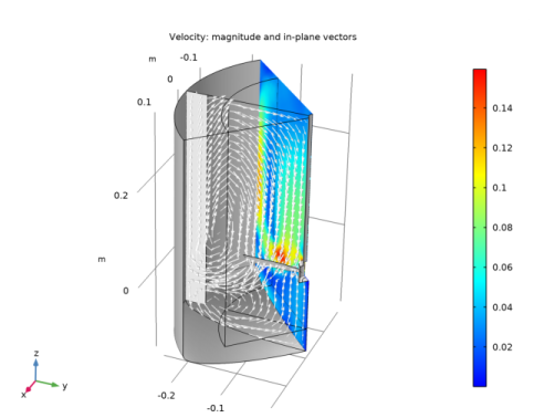
In the Settings window for 3D Plot Group, type Velocity: Magnitude and Vectors in the Label text field.
|
|
1
|
|
2
|
|
3
|
|
4
|
|
1
|
|
2
|
|
3
|
|
4
|
|
5
|
|
6
|
|
8
|
|
9
|
|
1
|
|
2
|
|
3
|
|
4
|
|
5
|
|
6
|
|
1
|
|
2
|
|
3
|
Locate the Expressions section. In the table, enter the following settings:
|
|
4
|
Click
|
|
1
|
|
2
|
|
3
|
Locate the Expressions section. In the table, enter the following settings:
|
|
4
|
Click
|
|
1
|
|
2
|
Browse to the model’s Application Libraries folder and double-click the file modular_mixer_ke.mph.
|
|
1
|
|
2
|
Right-click Component 1 (comp1)>Turbulent Flow, k-ε (spf) and choose Generate New Turbulence Model Interface.
|
|
3
|
In the Settings window for Generate New Turbulence Model Interface, locate the Turbulence Model Interface section.
|
|
4
|
|
5
|
|
1
|
|
2
|
|
3
|
|
1
|
|
2
|
|
3
|
|
4
|
|
1
|
|
2
|
|
3
|
|
1
|
|
2
|
|
3
|
|
1
|
In the Model Builder window, expand the Velocity: Magnitude and Vectors 1 node, then click Surface 2.
|
|
2
|
|
3
|
|
4
|
|
1
|
|
2
|
|
3
|
|
4
|
|
5
|
|
6
|
|
1
|
In the Model Builder window, under Results, Ctrl-click to select Velocity (spf2), Pressure (spf2), Wall Resolution (spf2), and Velocity: Magnitude and Vectors 1.
|
|
2
|
Right-click and choose Group.
|
|
1
|
In the Model Builder window, under Results, Ctrl-click to select Velocity (spf), Velocity: Magnitude and Vectors, and Wall Resolution (spf).
|
|
2
|
Right-click and choose Group.
|
|
1
|
|
2
|
|
3
|
|
4
|
|
5
|
Locate the Expressions section. In the table, enter the following settings:
|
|
6
|
Click
|
|
1
|
|
2
|
|
3
|
|
4
|
Locate the Expressions section. In the table, enter the following settings:
|
|
5
|
Click
|
|
1
|
In the Model Builder window, under Results>Derived Values, Ctrl-click to select Torque 1 and Power Draw 1.
|
|
2
|
Right-click and choose Group.
|
|
1
|
In the Model Builder window, under Results>Derived Values, Ctrl-click to select Torque and Power Draw.
|
|
2
|
Right-click and choose Group.
|