PDF

Residual Stress in a Thin-Film Resonator — 3D
Introduction
Almost all surface-micromachined thin films experience residual stress as a result of the fabrication process. The most common source of residual stress is thermal stress, which is caused by a change in temperature experienced during the fabrication sequence and also due to the difference in the coefficient of thermal expansion between the film and the substrate. This tutorial shows how to model thermal residual stress due to a temperature difference and how it changes the resonant frequency of a thin-film resonator. The substrate is not included in the model and it is also assumed that at a given state (which indicates a particular step of the process sequence), the temperature is uniform throughout the cantilever.
Figure 1: A thin-film resonator with four straight cantilever beam springs.
The tutorial investigates two design choices; a resonator with straight cantilevers (Figure 1) and another one with folded cantilevers (Figure 2). For each of the designs, the resonant frequency is computed for the cases when the structure is unstressed and when it is subjected to a residual thermal stress. The results obtained from these 3D models can be compared with analytical solutions by referring to the Application Libraries tutorial Residual Stress in a Thin-Film Resonator — 2D.
Figure 2: A thin-film resonator with four folded cantilever beam springs.
Model Definition
This tutorial uses the dimensions and material properties presented in Table 1 and Table 2. These values were obtained from the example in Chapter 27.2.5 in Ref. 1. This simulation models thermal residual stress using the Thermal Expansion feature in the Solid Mechanics interface. The coefficient of thermal expansion is computed by assuming a residual stress of 50 MPa in the straight cantilevers, a film deposition temperature of 605°C (see Chapter 16.13.2.3 in Ref. 1) and a room temperature of 25°C.
200 μm
170 μm
10 μm
146 μm
250 μm
2 μm
2 μm
2 μm
2 μm
120 μm
T0
605oC
T1
25oC
In order to determine the eigenfrequencies for the case with residual stress, a Prestressed-Eigenfrequency Study is used. This predefined study type first solves for a static thermal expansion problem to compute the residual stress. The solution of this static problem is then used to create a shift in the linearization point around which the eigenfrequencies are then computed. This approach accurately computes the shift in eigenfrequency by accounting for the stress-stiffening effect.
Results and Discussion
Table 3 summarizes the resonant frequencies for the first in-plane bending eigenmode. The solutions from the 3D models are compared with those obtained from a 2D plane-stress model available in the Application Libraries tutorial Residual Stress in a Thin-Film Resonator — 2D. As the table shows, the resonant frequency for the straight cantilevers increases significantly when the model includes residual stress. As expected, the stress sensitivity of the resonant frequency is reduced by folding the cantilevers. The results from the 3D models agree closely with those obtained from the 2D models. This indicates that such thin-film resonators can be efficiently modeled using a 2D plane-stress approach.
Note that for the 2D models, the first (lowest) eigenmode is the in-plane bending mode. However for the 3D models, the first (lowest) eigenmode is an out-of-plane torsional mode that you see in the default plot when you solve the Eigenfrequency study. The desired in-plane bending mode is the second eigenmode in the list of computed solutions. Hence, the main advantage of the 3D model is in finding any eigenmode where the resonator deforms largely in the out-of-plane direction.
Figure 3 and Figure 4 show the first in-plane bending resonance mode for the unstressed resonator with straight and folded cantilevers respectively.
Figure 3: The first in-plane bending eigenmode of the unstressed resonator with straight cantilevers.
Figure 4: The first in-plane bending eigenmode of the unstressed resonator with folded cantilevers.
Figure 5 and Figure 7 show the first in-plane bending resonance mode for the resonator with straight and folded cantilevers respectively when they have a residual thermal stress.
Figure 5: The first in-plane bending eigenmode of the resonator with straight cantilevers having residual thermal stress.
Figure 6: Residual thermal stress in the resonator with straight cantilevers when it is cooled from 605°C to 25°C.
Figure 6 and Figure 8 show the residual thermal stress (von Mises stress) distribution in the resonator with straight and folded cantilevers respectively when they are cooled from 605°C to 25°C. Figure 6 shows that the residual stress is almost uniform in the straight cantilever and is about 49 MPa. Figure 8 shows that the folded configuration significantly reduces the residual stress build-up. In this case the residual stress is around 2 MPa in most part of the cantilever except near the fixed end where it is close to 44 MPa.
Figure 7: The first in-plane bending eigenmode of the resonator with folded cantilevers having residual thermal stress.
Figure 8: Residual thermal stress in the resonator with folded cantilevers when it is cooled from 605°C to 25°C.
Reference
1. M. Gad-el-Hak, ed., The MEMS Handbook, CRC Press, London, 2002, ch. 16.12 and 27.2.5.
Application Library path: MEMS_Module/Actuators/residual_stress_resonator_3d
Modeling Instructions.
From the File menu, choose New.
New
In the New window, click  Model Wizard.
Model Wizard
1
In the Model Wizard window, click  3D.
2
In the Select Physics tree, select Structural Mechanics>Solid Mechanics (solid).
3
Click Add.
4
Click  Study.
5
In the Select Study tree, select General Studies>Eigenfrequency.
6
Load in the required global parameters. As well as defining some model variables, these values are used later for comparison between the model and the analytical solution.
Global Definitions
Parameters 1
1
In the Model Builder window, under Global Definitions click Parameters 1.
2
In the Settings window for Parameters, locate the Parameters section.
3
Click  Load from File.
4
First create a component to model the resonator with straight cantilevers. For convenience, the device geometry will be inserted from an existing file. You can read the instructions for creating the geometry in the Appendix — Geometry Instructions.
Geometry 1
1
In the Geometry toolbar, click  Insert Sequence.
2
3
In the Insert Sequence from File dialog box, click OK.
4
In the Geometry toolbar, click  Build All.
Next set up the required solid mechanics physics for the problem by adding a Thermal Expansion sub-feature and specifying the fixed boundaries.
Solid Mechanics (solid)
Linear Elastic Material 1
In the Model Builder window, under Component 1 (comp1)>Solid Mechanics (solid) click Linear Elastic Material 1.
Thermal Expansion 1
1
In the Physics toolbar, click  Attributes and choose Thermal Expansion.
2
In the Settings window for Thermal Expansion, locate the Model Input section.
3
From the T list, choose User defined. In the associated text field, type T0.
4
Click  Go to Source.
Global Definitions
Default Model Inputs
1
In the Model Builder window, under Global Definitions click Default Model Inputs.
2
In the Settings window for Default Model Inputs, locate the Browse Model Inputs section.
3
Find the Expression for remaining selection subsection. In the Volume reference temperature text field, type T1.
The reference strain for thermal expansion is now T1. This value will be common to all thermal expansion features in the model.
Solid Mechanics (solid)
Fixed Constraint 1
1
In the Physics toolbar, click  Boundaries and choose Fixed Constraint.
2
In the Settings window for Fixed Constraint, locate the Boundary Selection section.
3
Click  Paste Selection.
4
In the Paste Selection dialog box, type 7,15,21,29 in the Selection text field.
5
Now add a new material to the component in order to define the required physical properties of the device.
Materials
Material 1 (mat1)
1
In the Model Builder window, under Component 1 (comp1) right-click Materials and choose Blank Material.
2
In the Settings window for Material, locate the Material Contents section.
3
Configure a suitable mesh, a Mapped and swept mesh is appropriate for this device geometry.
Mesh 1
Mapped 1
1
In the Mesh toolbar, click  Boundary and choose Mapped.
2
In the Settings window for Mapped, locate the Boundary Selection section.
3
Click  Paste Selection.
4
In the Paste Selection dialog box, type 4,9,14,23,28 in the Selection text field.
5
Distribution 1
1
Right-click Mapped 1 and choose Distribution.
2
In the Settings window for Distribution, locate the Edge Selection section.
3
Click  Paste Selection.
4
In the Paste Selection dialog box, type 16,21,44,49 in the Selection text field.
5
6
In the Settings window for Distribution, locate the Distribution section.
7
In the Number of elements text field, type 2.
Size
1
In the Model Builder window, click Size.
2
In the Settings window for Size, locate the Element Size section.
3
From the Predefined list, choose Extra fine.
Swept 1
In the Mesh toolbar, click  Swept.
Distribution 1
1
Right-click Swept 1 and choose Distribution.
2
In the Settings window for Distribution, locate the Distribution section.
3
In the Number of elements text field, type 2.
4
Click  Build All.
Add a second component to model the resonator with folded cantilevers. As with the first component, the device geometry will be inserted for convenience.
Add Component
1
In the Model Builder window, right-click the root node and choose Add Component>3D.
2
In the Geometry toolbar, click  Insert Sequence.
3
4
In the Insert Sequence from File dialog box, select Geometry 2 in the Select geometry sequence to insert list.
5
Geometry 2
1
In the Geometry toolbar, click  Build All.
Now the solid mechanics physics can be configured, as with the first component. In addition, a material will be added to define the required properties of the second device and an appropriate mesh will be created.
Add Physics
1
In the Home toolbar, click  Add Physics to open the Add Physics window.
2
Go to the Add Physics window.
3
In the tree, select Structural Mechanics>Solid Mechanics (solid).
4
Click Add to Component 2 in the window toolbar.
5
In the Home toolbar, click  Add Physics to close the Add Physics window.
Solid Mechanics 2 (solid2)
Linear Elastic Material 1
In the Model Builder window, under Component 2 (comp2)>Solid Mechanics 2 (solid2) click Linear Elastic Material 1.
Thermal Expansion 1
1
In the Physics toolbar, click  Attributes and choose Thermal Expansion.
2
In the Settings window for Thermal Expansion, locate the Model Input section.
3
From the T list, choose User defined. In the associated text field, type T0.
Fixed Constraint 1
1
In the Physics toolbar, click  Boundaries and choose Fixed Constraint.
2
In the Settings window for Fixed Constraint, locate the Boundary Selection section.
3
Click  Paste Selection.
4
In the Paste Selection dialog box, type 46,48,68,70 in the Selection text field.
5
Materials
Material 2 (mat2)
1
In the Model Builder window, under Component 2 (comp2) right-click Materials and choose Blank Material.
2
In the Settings window for Material, locate the Material Contents section.
3
Mesh 2
Mapped 1
1
In the Mesh toolbar, click  Boundary and choose Mapped.
2
In the Settings window for Mapped, locate the Boundary Selection section.
3
Click  Paste Selection.
4
In the Paste Selection dialog box, type 4,9,13,18,22,27,36,41,45,50,54,63,67,72,76,81,88,93,97,102,106 in the Selection text field.
5
Distribution 1
1
Right-click Mapped 1 and choose Distribution.
2
In the Settings window for Distribution, locate the Edge Selection section.
3
Click  Paste Selection.
4
In the Paste Selection dialog box, type 12,21,26,30,73,78,104,113,118,122,161,166 in the Selection text field.
5
6
In the Settings window for Distribution, locate the Distribution section.
7
In the Number of elements text field, type 2.
Swept 1
In the Mesh toolbar, click  Swept.
Distribution 1
1
Right-click Swept 1 and choose Distribution.
2
In the Settings window for Distribution, locate the Distribution section.
3
In the Number of elements text field, type 2.
Size
1
In the Model Builder window, click Size.
2
In the Settings window for Size, locate the Element Size section.
3
From the Predefined list, choose Extra fine.
4
Click  Build All.
In order to perform the required computations four studies are required. The first two studies, one for each of the components, are for the case of zero-stress. These studies require one Eigenfrequency solver step, which will be used to calculate the eigenfrequency and mode of each resonator.
Study 1 - Straight Cantilever, No Stress
1
In the Model Builder window, right-click Study 1 and choose Rename.
2
In the Rename Study dialog box, type Study 1 - Straight Cantilever, No Stress in the New label text field.
3
Step 1: Eigenfrequency
1
In the Model Builder window, under Study 1 - Straight Cantilever, No Stress click Step 1: Eigenfrequency.
2
In the Settings window for Eigenfrequency, locate the Physics and Variables Selection section.
3
In the table, clear the Solve for check box for Solid Mechanics 2 (solid2).
Add Study
1
In the Home toolbar, click  Add Study to open the Add Study window.
2
Go to the Add Study window.
3
Find the Studies subsection. In the Select Study tree, select General Studies>Eigenfrequency.
4
Click Add Study in the window toolbar.
5
In the Home toolbar, click  Add Study to close the Add Study window.
Study 2 - Folded Cantilever, No Stress
1
In the Model Builder window, right-click Study 2 and choose Rename.
2
In the Rename Study dialog box, type Study 2 - Folded Cantilever, No Stress in the New label text field.
3
Step 1: Eigenfrequency
1
In the Model Builder window, click Step 1: Eigenfrequency.
2
In the Settings window for Eigenfrequency, locate the Physics and Variables Selection section.
3
In the table, clear the Solve for check box for Solid Mechanics (solid).
The second two studies require two study steps: an initial Stationary study step is used to calculate the residual thermal stress due to the difference between the fabrication and operation temperatures; the solution to this step is then used to shift the linerization point around which the eigenfrequenies are computed in a subsequent Eigenfrequency study step. Prestressed Analysis, Eigenfrequency studies are used as this study type contains the required study steps by default.
Add Study
1
In the Home toolbar, click  Add Study to open the Add Study window.
2
Go to the Add Study window.
3
Find the Studies subsection. In the Select Study tree, select Preset Studies for Selected Physics Interfaces>Eigenfrequency, Prestressed.
4
Click Add Study in the window toolbar.
5
In the Home toolbar, click  Add Study to close the Add Study window.
Study 3 - Straight Cantilever, Residual Stress
1
In the Model Builder window, right-click Study 3 and choose Rename.
2
In the Rename Study dialog box, type Study 3 - Straight Cantilever, Residual Stress in the New label text field.
3
Step 1: Stationary
1
In the Model Builder window, under Study 3 - Straight Cantilever, Residual Stress click Step 1: Stationary.
2
In the Settings window for Stationary, locate the Physics and Variables Selection section.
3
In the table, clear the Solve for check box for Solid Mechanics 2 (solid2).
Step 2: Eigenfrequency
1
In the Model Builder window, click Step 2: Eigenfrequency.
2
In the Settings window for Eigenfrequency, locate the Physics and Variables Selection section.
3
In the table, clear the Solve for check box for Solid Mechanics 2 (solid2).
Add Study
1
In the Home toolbar, click  Add Study to open the Add Study window.
2
Go to the Add Study window.
3
Find the Studies subsection. In the Select Study tree, select Preset Studies for Selected Physics Interfaces>Eigenfrequency, Prestressed.
4
Click Add Study in the window toolbar.
5
In the Home toolbar, click  Add Study to close the Add Study window.
Study 4 - Folded Cantilever, Residual Stress
1
In the Model Builder window, right-click Study 4 and choose Rename.
2
In the Rename Study dialog box, type Study 4 - Folded Cantilever, Residual Stress in the New label text field.
3
Step 1: Stationary
1
In the Model Builder window, under Study 4 - Folded Cantilever, Residual Stress click Step 1: Stationary.
2
In the Settings window for Stationary, locate the Physics and Variables Selection section.
3
In the table, clear the Solve for check box for Solid Mechanics (solid).
Step 2: Eigenfrequency
1
In the Model Builder window, click Step 2: Eigenfrequency.
2
In the Settings window for Eigenfrequency, locate the Physics and Variables Selection section.
3
In the table, clear the Solve for check box for Solid Mechanics (solid).
The studies can now be solved and the results visualized.
Study 1 - Straight Cantilever, No Stress
In the Home toolbar, click  Compute.
Results
Straight Cantilever, No Stress
1
Right-click Results>Mode Shape (solid) and choose Rename.
2
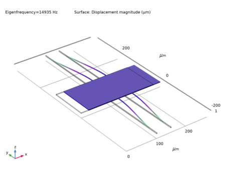
In the Rename 3D Plot Group dialog box, type Straight Cantilever, No Stress in the New label text field.
3
4
In the Settings window for 3D Plot Group, locate the Data section.
5
From the Eigenfrequency (Hz) list, choose 14935.
6
In the Straight Cantilever, No Stress toolbar, click  Plot.
Study 2 - Folded Cantilever, No Stress
In the Home toolbar, click  Compute.
Results
Folded Cantilever, No Stress
1
Right-click Results>Mode Shape (solid2) and choose Rename.
2
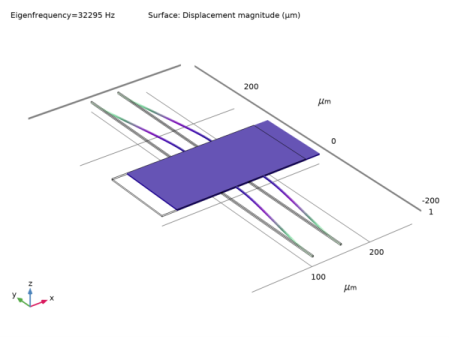
In the Rename 3D Plot Group dialog box, type Folded Cantilever, No Stress in the New label text field.
3
4
In the Settings window for 3D Plot Group, locate the Data section.
5
From the Eigenfrequency (Hz) list, choose 14199.
6
In the Folded Cantilever, No Stress toolbar, click  Plot.
Study 3 - Straight Cantilever, Residual Stress
In the Home toolbar, click  Compute.
Results
Straight Cantilever, Residual Stress
1
Right-click Results>Mode Shape (solid) and choose Rename.
2
In the Rename 3D Plot Group dialog box, type Straight Cantilever, Residual Stress in the New label text field.
3
4
In the Settings window for 3D Plot Group, locate the Data section.
5
From the Eigenfrequency (Hz) list, choose 32295.
6
In the Straight Cantilever, Residual Stress toolbar, click  Plot.
Study 4 - Folded Cantilever, Residual Stress
In the Home toolbar, click  Compute.
Results
Folded Cantilever, Residual Stress
1
Right-click Results>Mode Shape (solid2) and choose Rename.
2
In the Rename 3D Plot Group dialog box, type Folded Cantilever, Residual Stress in the New label text field.
3
4
In the Settings window for 3D Plot Group, locate the Data section.
5
From the Eigenfrequency (Hz) list, choose 14302.
6
In the Folded Cantilever, Residual Stress toolbar, click  Plot.
Residual Stress in Straight Cantilever
1
In the Home toolbar, click  Add Plot Group and choose 3D Plot Group.
2
Right-click 3D Plot Group 5 and choose Rename.
3
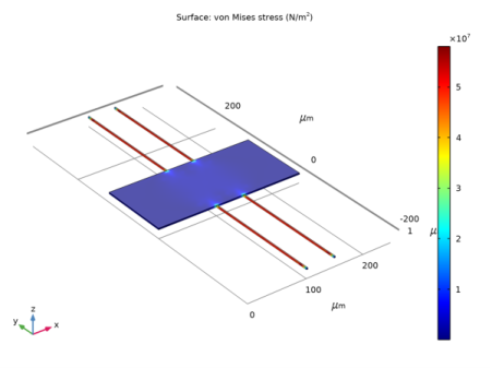
In the Rename 3D Plot Group dialog box, type Residual Stress in Straight Cantilever in the New label text field.
4
5
In the Settings window for 3D Plot Group, locate the Data section.
6
From the Dataset list, choose Study 3 - Straight Cantilever, Residual Stress/Solution Store 1 (7) (sol4).
Surface 1
1
Right-click Residual Stress in Straight Cantilever and choose Surface.
2
In the Settings window for Surface, locate the Expression section.
3
In the Expression text field, type solid.mises.
4
In the Residual Stress in Straight Cantilever toolbar, click  Plot.
Residual Stress in Folded Cantilever
1
In the Home toolbar, click  Add Plot Group and choose 3D Plot Group.
2
Right-click 3D Plot Group 6 and choose Rename.
3
In the Rename 3D Plot Group dialog box, type Residual Stress in Folded Cantilever in the New label text field.
4
5
In the Settings window for 3D Plot Group, locate the Data section.
6
From the Dataset list, choose Study 4 - Folded Cantilever, Residual Stress/Solution Store 2 (12) (sol6).
Surface 1
1
Right-click Residual Stress in Folded Cantilever and choose Surface.
2
In the Settings window for Surface, locate the Expression section.
3
In the Expression text field, type solid2.mises.
4
In the Residual Stress in Folded Cantilever toolbar, click  Plot.
 
Appendix — Geometry Instructions
From the File menu, choose New.
New
In the New window, click  Model Wizard.
Model Wizard
1
In the Model Wizard window, click  3D.
2
In the Select Physics tree, select Structural Mechanics>Solid Mechanics (solid).
3
Click Add.
4
Geometry 1
1
In the Model Builder window, under Component 1 (comp1) click Geometry 1.
2
In the Settings window for Geometry, locate the Units section.
3
From the Length unit list, choose µm.
Work Plane 1 (wp1)
1
In the Geometry toolbar, click  Work Plane.
2
In the Settings window for Work Plane, click  Show Work Plane.
Work Plane 1 (wp1)>Plane Geometry
In the Model Builder window, click Plane Geometry.
Work Plane 1 (wp1)>Rectangle 1 (r1)
1
In the Work Plane toolbar, click  Rectangle.
2
In the Settings window for Rectangle, locate the Size and Shape section.
3
In the Width text field, type 250.
4
In the Height text field, type 120.
Work Plane 1 (wp1)>Rectangle 2 (r2)
1
In the Work Plane toolbar, click  Rectangle.
2
In the Settings window for Rectangle, locate the Size and Shape section.
3
In the Width text field, type 2.
4
In the Height text field, type 200.
5
Locate the Position section. In the xw text field, type 100.
6
In the yw text field, type 120.
Work Plane 1 (wp1)>Array 1 (arr1)
1
In the Work Plane toolbar, click  Transforms and choose Array.
2
3
In the Settings window for Array, locate the Size section.
4
In the xw size text field, type 2.
5
In the yw size text field, type 2.
6
Locate the Displacement section. In the xw text field, type 48.
7
In the yw text field, type -320.
Work Plane 1 (wp1)>Plane Geometry
In the Work Plane toolbar, click  Build All.
Extrude 1 (ext1)
1
In the Model Builder window, right-click Geometry 1 and choose Extrude.
2
In the Settings window for Extrude, locate the Distances section.
3
4
Click  Build All Objects.
Add Component
In the Model Builder window, right-click the root node and choose Add Component>3D.
Geometry 2
1
In the Settings window for Geometry, locate the Units section.
2
From the Length unit list, choose µm.
Work Plane 1 (wp1)
1
In the Geometry toolbar, click  Work Plane.
2
In the Settings window for Work Plane, click  Show Work Plane.
Work Plane 1 (wp1)>Plane Geometry
In the Model Builder window, click Plane Geometry.
Work Plane 1 (wp1)>Rectangle 1 (r1)
1
In the Work Plane toolbar, click  Rectangle.
2
In the Settings window for Rectangle, locate the Size and Shape section.
3
In the Width text field, type 250.
4
In the Height text field, type 120.
Work Plane 1 (wp1)>Rectangle 2 (r2)
1
In the Work Plane toolbar, click  Rectangle.
2
In the Settings window for Rectangle, locate the Size and Shape section.
3
In the Width text field, type 2.
4
In the Height text field, type 172.
5
Locate the Position section. In the xw text field, type 100.
6
In the yw text field, type 120.
Work Plane 1 (wp1)>Rectangle 3 (r3)
1
In the Work Plane toolbar, click  Rectangle.
2
In the Settings window for Rectangle, locate the Size and Shape section.
3
In the Width text field, type 12.
4
In the Height text field, type 2.
5
Locate the Position section. In the xw text field, type 100.
6
In the yw text field, type 290.
Work Plane 1 (wp1)>Rectangle 4 (r4)
1
In the Work Plane toolbar, click  Rectangle.
2
In the Settings window for Rectangle, locate the Size and Shape section.
3
In the Width text field, type 2.
4
In the Height text field, type 148.
5
Locate the Position section. In the xw text field, type 110.
6
In the yw text field, type 144.
Work Plane 1 (wp1)>Mirror 1 (mir1)
1
In the Work Plane toolbar, click  Transforms and choose Mirror.
2
Click the  Zoom Extents button in the Graphics toolbar.
3
Select the objects r2, r3, and r4 only.
4
In the Settings window for Mirror, locate the Input section.
5
Select the Keep input objects check box.
6
Locate the Point on Line of Reflection section. In the xw text field, type 125.
Work Plane 1 (wp1)>Mirror 2 (mir2)
1
In the Work Plane toolbar, click  Transforms and choose Mirror.
2
Select the objects mir1(1), mir1(2), mir1(3), r2, r3, and r4 only.
3
In the Settings window for Mirror, locate the Input section.
4
Select the Keep input objects check box.
5
Locate the Point on Line of Reflection section. In the yw text field, type 60.
6
Locate the Normal Vector to Line of Reflection section. In the xw text field, type 0.
7
In the yw text field, type 1.
Extrude 1 (ext1)
1
In the Model Builder window, right-click Geometry 2 and choose Extrude.
2
In the Settings window for Extrude, locate the Distances section.
3
4
Click  Build All Objects.