|
|
|
|
•
|
A payload of 1000 kg at the tip of the crane.
|
|
1
|
|
2
|
|
3
|
Click Add.
|
|
4
|
Click
|
|
5
|
|
6
|
Click
|
|
1
|
|
2
|
|
3
|
Click Browse.
|
|
4
|
Browse to the model’s Application Libraries folder and double-click the file truck_mounted_crane.mphbin.
|
|
5
|
Click Import.
|
|
1
|
|
2
|
|
3
|
|
4
|
|
5
|
|
1
|
|
2
|
|
3
|
|
4
|
|
5
|
|
1
|
In the Model Builder window, under Component 1 (comp1) right-click Multibody Dynamics (mbd) and choose Rigid Domain.
|
|
2
|
|
2
|
|
1
|
|
2
|
|
3
|
|
4
|
|
5
|
|
1
|
In the Model Builder window, expand the Hinge Base-Boom1 node, then click Center of Joint: Boundary 1.
|
|
1
|
|
2
|
|
3
|
|
4
|
|
5
|
|
1
|
In the Model Builder window, expand the Hinge Base-Cylinder1 node, then click Center of Joint: Boundary 1.
|
|
1
|
|
2
|
|
3
|
|
4
|
|
5
|
|
1
|
In the Model Builder window, expand the Hinge Base-Link1 node, then click Center of Joint: Boundary 1.
|
|
1
|
|
2
|
|
3
|
|
4
|
|
5
|
|
1
|
In the Model Builder window, expand the Hinge Boom1-Link2 node, then click Center of Joint: Boundary 1.
|
|
1
|
|
2
|
|
3
|
|
4
|
|
5
|
|
1
|
In the Model Builder window, expand the Slot Link1-Link2 node, then click Center of Joint: Boundary 1.
|
|
1
|
|
2
|
|
3
|
|
1
|
|
2
|
In the Settings window for Prismatic Joint, type Prismatic Cylinder1-Piston1 in the Label text field.
|
|
3
|
|
4
|
|
5
|
|
6
|
|
7
|
|
1
|
In the Model Builder window, expand the Prismatic Cylinder1-Piston1 node, then click Center of Joint: Boundary 1.
|
|
1
|
|
1
|
Right-click and choose Duplicate.
|
|
2
|
|
3
|
|
4
|
|
1
|
In the Model Builder window, expand the Hinge Boom1-Boom2 node, then click Center of Joint: Boundary 1.
|
|
2
|
|
3
|
|
1
|
In the Model Builder window, under Component 1 (comp1)>Multibody Dynamics (mbd) click Hinge Base-Cylinder1.1.
|
|
2
|
|
3
|
|
4
|
|
1
|
In the Model Builder window, expand the Hinge Boom1-Cylinder2 node, then click Center of Joint: Boundary 1.
|
|
2
|
|
3
|
|
1
|
In the Model Builder window, under Component 1 (comp1)>Multibody Dynamics (mbd) click Hinge Base-Link1.1.
|
|
2
|
|
3
|
|
4
|
|
1
|
In the Model Builder window, expand the Hinge Boom1-Link3 node, then click Center of Joint: Boundary 1.
|
|
2
|
|
3
|
|
1
|
In the Model Builder window, under Component 1 (comp1)>Multibody Dynamics (mbd) click Hinge Boom1-Link2.1.
|
|
2
|
|
3
|
|
4
|
|
1
|
In the Model Builder window, expand the Hinge Boom2-Link4 node, then click Center of Joint: Boundary 1.
|
|
2
|
|
3
|
|
1
|
In the Model Builder window, under Component 1 (comp1)>Multibody Dynamics (mbd) click Slot Link1-Link2.1.
|
|
2
|
|
3
|
|
4
|
|
1
|
In the Model Builder window, expand the Slot Link3-Link4 node, then click Center of Joint: Boundary 1.
|
|
2
|
|
3
|
|
1
|
In the Model Builder window, under Component 1 (comp1)>Multibody Dynamics (mbd) click Slot Link1-Piston1.1.
|
|
2
|
|
3
|
|
4
|
|
1
|
In the Model Builder window, expand the Slot Link3-Piston2 node, then click Center of Joint: Boundary 1.
|
|
2
|
|
3
|
|
1
|
In the Model Builder window, under Component 1 (comp1)>Multibody Dynamics (mbd) click Prismatic Cylinder1-Piston1.1.
|
|
2
|
In the Settings window for Prismatic Joint, type Prismatic Cylinder2-Piston2 in the Label text field.
|
|
3
|
|
4
|
|
5
|
|
1
|
In the Model Builder window, expand the Prismatic Cylinder2-Piston2 node, then click Center of Joint: Boundary 1.
|
|
2
|
|
3
|
|
1
|
|
2
|
|
3
|
|
1
|
|
2
|
In the Settings window for Prismatic Joint, type Prismatic Boom2-Extension1 in the Label text field.
|
|
3
|
|
4
|
|
5
|
|
6
|
|
1
|
In the Model Builder window, expand the Prismatic Boom2-Extension1 node, then click Center of Joint: Boundary 1.
|
|
1
|
|
2
|
In the Settings window for Prismatic Joint, type Prismatic Extension1-Extension2 in the Label text field.
|
|
3
|
|
4
|
|
5
|
|
6
|
|
1
|
In the Model Builder window, expand the Prismatic Extension1-Extension2 node, then click Center of Joint: Boundary 1.
|
|
1
|
|
2
|
In the Settings window for Prismatic Joint, type Prismatic Extension2-Extension3 in the Label text field.
|
|
3
|
|
4
|
|
5
|
|
6
|
|
1
|
In the Model Builder window, expand the Prismatic Extension2-Extension3 node, then click Center of Joint: Boundary 1.
|
|
3
|
|
4
|
|
1
|
|
2
|
|
3
|
|
1
|
|
3
|
|
4
|
|
5
|
|
1
|
|
2
|
|
1
|
|
2
|
In the Show More Options dialog box, in the tree, select the check box for the node Physics>Equation-Based Contributions.
|
|
3
|
Click OK.
|
|
1
|
|
2
|
|
4
|
|
5
|
|
6
|
Click
|
|
7
|
|
8
|
Click OK.
|
|
9
|
|
1
|
|
2
|
|
3
|
|
4
|
Click to expand the Reaction Force Settings section. Select the Apply reaction only on joint variables check box.
|
|
1
|
|
2
|
|
3
|
|
4
|
Locate the Reaction Force Settings section. Select the Apply reaction only on joint variables check box.
|
|
1
|
|
2
|
|
3
|
|
1
|
|
2
|
|
3
|
|
1
|
|
2
|
|
3
|
|
1
|
|
2
|
|
1
|
|
2
|
|
1
|
|
2
|
|
3
|
|
4
|
|
1
|
|
2
|
|
3
|
|
4
|
|
6
|
|
1
|
|
2
|
|
3
|
|
4
|
|
5
|
Browse to the model’s Application Libraries folder and double-click the file truck_mounted_crane_solparam.txt.
|
|
6
|
|
1
|
|
2
|
|
3
|
In the Model Builder window, expand the Study 1>Solver Configurations>Solution 1 (sol1)>Dependent Variables 1 node, then click comp1.ODE1.
|
|
4
|
|
5
|
|
6
|
|
7
|
|
8
|
|
9
|
|
1
|
|
2
|
|
3
|
Select the Plot check box.
|
|
4
|
|
1
|
|
2
|
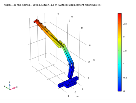
From the Parameter value (Angle1 (rad),RelAng (rad),ExtLen (m)) list, choose 9: Angle1=45 rad, RelAng=-30 rad, ExtLen=1.5 m.
|
|
3
|
|
4
|
|
1
|
|
2
|
|
1
|
|
2
|
|
4
|
|
5
|
|
6
|
|
1
|
|
2
|
|
3
|
|
4
|
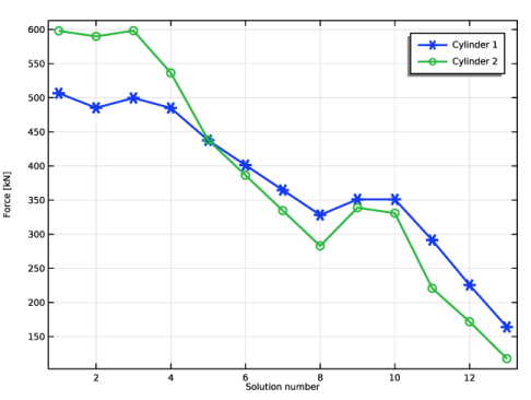
In the associated text field, type Force [kN].
|
|
5
|
|
6
|
|
1
|
|
2
|
|
1
|
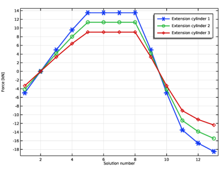
In the Model Builder window, expand the Boom cylinder forces 1 node, then click Results>Extension cylinder forces>Global 1.
|
|
2
|
|
4
|
|
1
|
|
2
|
|
1
|
|
2
|
|
4
|
|
5
|
|
6
|
|
1
|
|
2
|
|
3
|
|
4
|
|
5
|
In the associated text field, type Force [kN].
|
|
6
|
|
7
|
|
1
|
|
2
|
|
1
|
|
3
|
|
4
|
|
5
|
|
6
|
|
7
|
|
8
|
|
9
|
|
1
|
|
2
|
|
3
|
|
4
|
|
5
|