
|
|
|
|
•
|
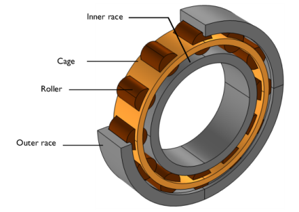
In this model, all components are modeled as rigid elements using the Rigid Domain nodes which can be created automatically using the Create Rigid Domains button in the Automated Model Setup section at the physics interface.
|
|
•
|
Joint nodes between rollers and cage can also be created automatically using the Create Joints button in the Automated Model Setup section at the physics interface. The automatic joint creation requires the geometry to be in assembly mode and Identity Boundary Pair nodes to be available in the Definitions.
|
|
1
|
|
2
|
|
3
|
Click Add.
|
|
4
|
Click
|
|
5
|
|
6
|
Click
|
|
1
|
|
2
|
|
3
|
|
4
|
Browse to the model’s Application Libraries folder and double-click the file roller_bearing_dynamics_parameters.txt.
|
|
1
|
|
2
|
|
3
|
|
4
|
Click Browse.
|
|
5
|
Browse to the model’s Application Libraries folder and double-click the file roller_bearing_dynamics.mphbin.
|
|
6
|
Click Import.
|
|
1
|
|
2
|
|
3
|
On the object imp1(2), select Domain 1 only.
|
|
4
|
|
5
|
|
1
|
|
2
|
|
3
|
On the object imp1(1), select Domain 1 only.
|
|
4
|
On the object imp1(15), select Domains 1–4 only.
|
|
5
|
|
6
|
|
7
|
Click Define custom colors.
|
|
9
|
Click Add to custom colors.
|
|
10
|
|
11
|
|
1
|
|
2
|
|
3
|
|
4
|
|
5
|
Click OK.
|
|
6
|
|
7
|
|
8
|
|
1
|
|
2
|
|
3
|
|
4
|
|
5
|
Click OK.
|
|
6
|
|
1
|
|
2
|
In the Settings window for Adjacent Selection, type Cage & Rollers Boundaries in the Label text field.
|
|
3
|
|
4
|
|
5
|
Click OK.
|
|
6
|
|
1
|
|
2
|
|
3
|
On the object imp1(15), select Domains 1–4 only.
|
|
4
|
|
1
|
|
2
|
|
3
|
|
4
|
|
5
|
Click OK.
|
|
6
|
|
7
|
|
8
|
|
1
|
|
2
|
In the Settings window for Complement Selection, type Boundaries without Outer Race in the Label text field.
|
|
3
|
|
4
|
|
5
|
|
6
|
Click OK.
|
|
7
|
|
1
|
|
2
|
|
3
|
|
4
|
|
5
|
|
6
|
|
7
|
On the object fin, select Domain 1 only.
|
|
1
|
In the Model Builder window, under Component 1 (comp1) right-click Definitions and choose Variables.
|
|
2
|
|
3
|
|
4
|
Browse to the model’s Application Libraries folder and double-click the file roller_bearing_dynamics_variables.txt.
|
|
1
|
|
2
|
|
3
|
|
4
|
Select the Cutoff check box.
|
|
1
|
|
2
|
|
3
|
|
4
|
|
5
|
|
1
|
|
2
|
In the Settings window for Multibody Dynamics, click Physics Node Generation in the upper-right corner of the Automated Model Setup section. From the menu, choose Create Rigid Domains.
|
|
1
|
|
2
|
|
1
|
|
2
|
|
1
|
|
2
|
In the Settings window for Prescribed Displacement/Rotation, locate the Prescribed Displacement at Center of Rotation section.
|
|
3
|
|
4
|
|
5
|
|
6
|
|
1
|
|
2
|
|
1
|
|
2
|
In the Settings window for Prescribed Displacement/Rotation, locate the Prescribed Displacement at Center of Rotation section.
|
|
3
|
|
4
|
|
5
|
Specify the Ω vector as
|
|
6
|
|
1
|
|
2
|
|
3
|
Specify the F vector as
|
|
4
|
|
5
|
In the Settings window for Multibody Dynamics, click Physics Node Generation in the upper-right corner of the Automated Model Setup section. From the menu, choose Create Joints.
|
|
1
|
|
2
|
|
3
|
|
4
|
|
5
|
|
6
|
|
7
|
|
8
|
|
9
|
|
1
|
|
2
|
|
3
|
|
4
|
|
1
|
In the Model Builder window, under Component 1 (comp1)>Multibody Dynamics (mbd), Ctrl-click to select Rigid Body Contact 1, Rigid Body Contact 2, Rigid Body Contact 3, Rigid Body Contact 4, Rigid Body Contact 5, Rigid Body Contact 6, Rigid Body Contact 7, Rigid Body Contact 8, Rigid Body Contact 9, Rigid Body Contact 10, Rigid Body Contact 11, and Rigid Body Contact 12.
|
|
2
|
Right-click and choose Group.
|
|
1
|
|
2
|
|
1
|
In the Model Builder window, expand the Roller-Inner Race Contact node, then click Rigid Body Contact 13.
|
|
2
|
|
3
|
|
4
|
|
5
|
|
1
|
Similar to the changes done for Rigid Body Contact 13, reset the inputs of other eleven Rigid Body Contact nodes using the information given in the table below.
|
|
2
|
|
3
|
|
4
|
|
1
|
|
2
|
|
3
|
|
4
|
|
1
|
|
2
|
|
3
|
|
1
|
|
2
|
|
3
|
In the Model Builder window, expand the Study 1>Solver Configurations>Solution 1 (sol1)>Time-Dependent Solver 1 node, then click Fully Coupled 1.
|
|
4
|
|
5
|
|
6
|
|
7
|
|
8
|
|
9
|
|
1
|
|
2
|
|
3
|
|
4
|
|
1
|
|
2
|
|
3
|
|
4
|
|
1
|
|
2
|
|
3
|
|
4
|
|
5
|
|
1
|
|
2
|
|
3
|
|
4
|
|
1
|
|
2
|
|
3
|
Click to expand the Selection section. Locate the Plot Settings section. From the View list, choose New view.
|
|
1
|
|
2
|
|
1
|
|
2
|
|
3
|
|
4
|
|
5
|
|
1
|
|
2
|
|
3
|
|
4
|
|
5
|
|
1
|
|
2
|
|
3
|
|
4
|
|
1
|
|
2
|
|
3
|
|
1
|
|
2
|
|
3
|
|
1
|
|
2
|
|
3
|
|
4
|
|
5
|
|
6
|
Select the Description check box.
|
|
7
|
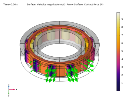
In the associated text field, type Contact force (N).
|
|
8
|
|
10
|
|
1
|
|
2
|
|
3
|
|
1
|
|
2
|
|
3
|
|
4
|
|
1
|
|
2
|
|
1
|
|
2
|
|
3
|
|
1
|
|
2
|
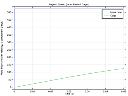
In the Settings window for 1D Plot Group, type Angular Speed [Inner Race & Cage] in the Label text field.
|
|
3
|
|
1
|
|
2
|
|
4
|
|
6
|
|
1
|
|
2
|
|
1
|
|
2
|
|
4
|
|
5
|
Locate the Legends section. In the table, enter the following settings:
|
|
6
|
|
1
|
|
2
|
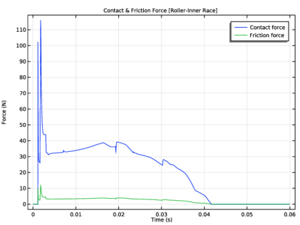
In the Settings window for 1D Plot Group, type Contact & Friction Force [Roller-Inner Race] in the Label text field.
|
|
1
|
In the Model Builder window, expand the Contact & Friction Force [Roller-Inner Race] node, then click Global 1.
|
|
2
|
|
3
|
|
5
|
|
1
|
|
2
|
|
3
|
|
4
|
In the associated text field, type Force (N).
|
|
5
|
|
1
|
|
2
|
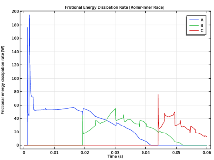
In the Settings window for 1D Plot Group, type Frictional Energy Dissipation Rate [Roller-Inner Race] in the Label text field.
|
|
1
|
In the Model Builder window, expand the Frictional Energy Dissipation Rate [Roller-Inner Race] node, then click Global 1.
|
|
2
|
|
3
|
|
5
|
|
1
|
|
2
|
|
3
|
|
4
|
|
1
|
|
2
|
|
1
|
|
2
|
|
3
|
|
5
|
|
6
|
|
7
|
|
8
|
|
1
|
|
2
|
|
1
|
|
2
|
|
3
|
|
1
|
|
2
|
|
3
|
|
1
|
|
2
|
|
3
|